• 12. Power and Precision
Motivating Scenario:
You’re designing a study and need to decide how big to make it. Too few samples, and a real effect could hide in the noise, but too many samples represent an unnecessary waste of time, money, and effort. Here we will think about design strategies to get the most information from your study, and how to decide how many samples you need
Learning Goals: By the end of this chapter, you should be able to:
- Describe how to design an experiment to decrease variability and increase precision.
- Recognize pseudoreplication, how to avoid it, and what to do about it.
- Know that you can plan for power and precision and recognize the R packages and webapps to plan a sample size with adequate statistical power.
- Explain why small effects require disproportionately larger samples to detect, and why reducing variance can substitute for collecting more data.
“You can’t stop sampling error, you can only hope to contain it.”
– Adapted from Dan Patrick catchphrase.
There is no stopping sampling error, the chance deviation between the true population parameter and our estimate from a sample. But, this does not mean that we are stuck wandering around with hopeless uncertainty. There are proven ways to minimize sampling error, which can be broken up into two types of strategies. We can aim to decrease variability, and/or increase the number of independent samples. I note that I introduced some of these ideas in our section on Sampling Better.
Decreasing variability
One simple way to increase the precision of an estimate is to decrease variability. We only have so much control over this, since some variability is natural – but there are things we can do to increase the precision of our estimated effect and minimize extraneous variation.
Increase measurement reliability
We cannot always measure the values of the explanatory or response variables with 100% accuracy. But we can take measures to increase the reliability of such measures. For example, in our RIL study, we measured the proportion of hybrid seeds on a RIL as the number of hybrids out of the eight seeds genotyped. Increasing the number of seeds genotyped would increase measurement reliability, and decrease variability.
Balanced design
Balance refers to the similarity in sample sizes across treatments. Say, for example, we wanted to estimate the difference in the proportion of hybrid seed on a total of fifty white- and pink-flowered parviflora RILs. If we had 50 pink RILs and 0 white RILs we would not be able to estimate this difference. Or if we had only a handful of white RILs our estimate for white would be noisy and so our estimated difference would be too. The best approach would be to equally split our efforts between white- and pink-flowered RILs. For a fixed total sample size, more balanced experiments decrease the uncertainty in mean differences between treatments.
Matching
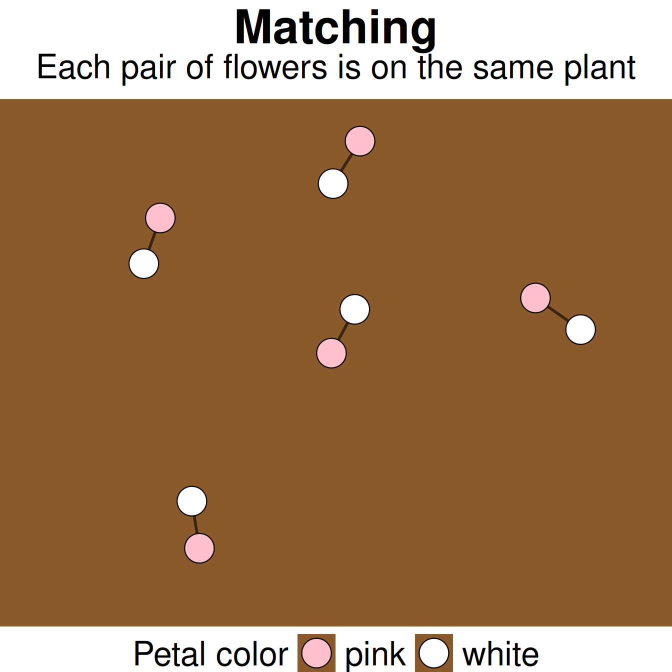
A standard experimental design is to randomize who gets the treatment and who gets the control. But we can do even better than that. When, e.g., pairs of individuals are matched to be nearly identical in every way except the treatment, we have more power to observe the effect of treatment. So, for example, if we could turn some flowers on the same plant pink and others white (Figure 1), we could remove the plant-to-plant variation in hybrid seed formation, and more precisely estimate the difference in hybrid formation between flower colors. This idea is statistically represented in the paired t-test, which we will soon encounter.
Blocking
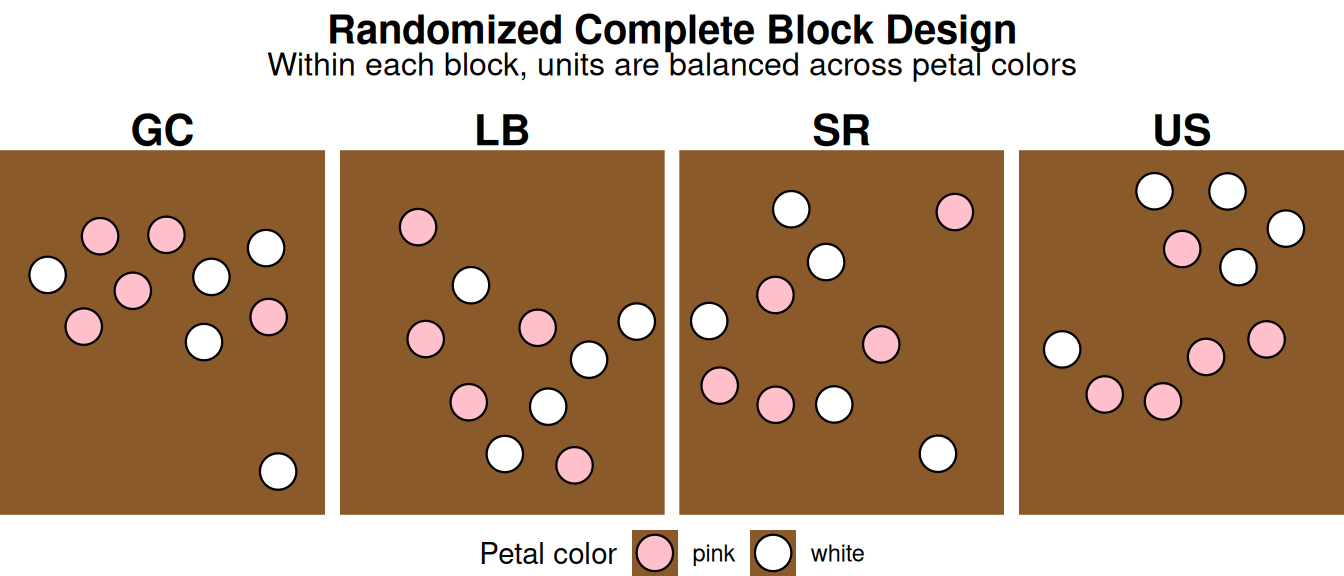
We can scale up the same principle behind matching to larger groups. Say we’re planting RILs at four different field sites. Of course, no two field sites are identical, they differ in e.g. soil properties, microclimate, pollinator community, etc. Randomly planting pink- and white-petaled RILs across sites isn’t the worst thing you could do, but it does add noise to our estimate. The site-to-site variation that has nothing to do with petal color or petal area will just add noise to our estimates. When blocking, we treat each site as a mini-experiment: planting a balanced set of RILs – both colors – at every site (Figure 2). That way, when we analyze the data, we can account for the differences between sites directly, instead of having them blur into the uncertainty around our treatment estimate. This approach, known as a Randomized Complete Block Design, is analyzed statistically by including site as a blocking factor in our model (often with multiple regression or mixed effect models), allowing us to estimate the effect of petal color or petal area after accounting for site-to-site differences.
Other techniques
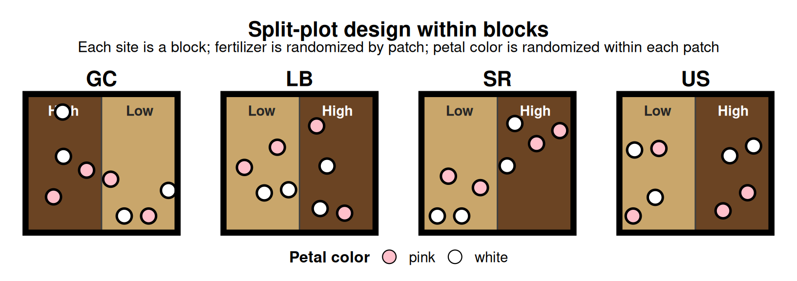
Blocking and matching are just two entries in a much bigger toolbox. Here I briefly introduce Split-plot designs (Figure 3) because I see them often. Split plots are used when one factor is hard to randomize at a fine scale. Say we also wanted to test whether more fertilizer changes hybridization rates, alongside our petal color comparison. Fertilizer leaks across a plot, so it can only be randomized at the patch level (not flower by flower) within each field site. This gives us two nested levels of randomization: (1) The random spread of pink and white within a patch, and (2) the randomly placed patches within field sites. In our analysis, we can then model these different sources of variability.
Eliminate (or model) non-independence
Our parviflora RIL study includes pseudoreplication. We have multiple observations of the same RIL in e.g. different field sites. In our scientific papers, we have modeled this non-independence, but this involves statistical techniques about one step further than we will get in this book. So for now, we simply note this non-independence, and move forward for the purposes of teaching and learning.
Pseudoreplication describes the case in which our replicates are not independent (see the earlier section on non-independent sampling). Ignoring pseudoreplication makes our estimate look far more precise than it really is.
The careful reader might notice an apparent contradiction. I just said that blocking (e.g. grouping RILs by site) and matching were good things, and then said to avoid pseudoreplication. Well, blocking and matching can be a good thing or not - the difference is whether that grouping gets modeled or ignored. Applying the appropriate statistical tools to a design with blocking allows us to use the nested structure to pull out site-to-site variance, and sharpen our estimate. By contrast, pseudoreplication without modelling this structure hides the noise instead of removing it. So when there is potential non-independence, be sure the unit of analysis matches our actual unit of randomization
Planning for power and precision
“Absence of evidence is not evidence of absence.”
– Often attributed to Carl Sagan (but others said it first)
We all know how to make estimates match true parameters – measure the entire population. But this is neither practical, nor smart (it’s a huge waste of time and energy). So a key question when you plan your experiment is, “how much certainty do you want in your estimate / how much power to reject the null do you want?”
As a BIOstats teacher, my key guidance is this: aim for an estimate that’s slightly more precise than you’d strictly need to detect a biologically meaningful difference or inform a policy decision – precise enough to give yourself some comfort, but not so precise that you’re chasing precision for its own sake. Here’s a rough guide to help:
- How precise an estimate do we need for our biological story? In some cases small differences matter a lot; in other cases, ballpark estimates are good enough. It’s your job as the researcher to know what your question requires.
- What effect size is worth knowing about? The null hypothesis is basically always false. With an infinite sample size, we’d probably always reject it. But in many cases the true population parameter is close enough to zero that the null hypothesis might as well be true. Again, it’s your job as a researcher to decide what size of effect you’d like to be able to detect.
- How much variability do we expect between measurements? Your biological knowledge is required here too (or you can consider the difference relative to variability when thinking about precision and effect size together).
Once you have a sense of the answers to these questions, we can use the tools below to find the appropriate sample size for your study.
Power: A brief review
Because estimates are influenced by chance, our ability to correctly reject a false null hypothesis (or not) is probabilistic. Power, the probability that we correctly reject a false null hypothesis is influenced by two factors:
The “effect size” – that is the difference between the true parameter and the null, and
The precision of our estimate. This itself is influenced by the nature of the world (which we cannot control) by choices in experiment design (see above), including sample size (see below).
Estimating an appropriate sample size
The power to reject the null: We know that rejecting the null hypothesis is not the goal of statistics. Still, if we are spending time and effort on a study, it is worth considering if that study would be able to identify biologically meaningful differences between treatments if they exist. We use power analyses to find the sample size needed for a study to have a good chance of rejecting a false null hypothesis. A power analysis basically finds the sample size necessary so that the sampling distribution of your experiment has:
- Some specified power to differentiate between the null model and the smallest effect size you’d like to be able to identify, and/or
- Some specified probability of being as precise, or more precise, than you want.
The traditional target power researchers shoot for is 80%, but in my opinion that’s quite low – aiming for 90% power seems more reasonable.
Mathematical intuition
The sample size needed to reject the null for some desired level of power, scales roughly as \(n \propto \frac{\sigma^2}{\text{effect}^2}\). So
Finding a small effect requires a huge sample. The required sample size grows as the square of one over the effect size. This means that it takes a hundredfold increase in n to find an effect that is ten times smaller. So if you really want to find a small effect you will need to invest a lot of time, energy, and money.
Reducing noise is as good as adding data. Variance (\(\sigma^2\)), enters the formula linearly. So using the techniques above to decrease variance provides the same gain in power as doubling your sample size, and can often come with less expense and effort.
Computational approaches
There are both online tools (e.g., this one from UBC) and R packages (the pwr package is most popular) to find the power you need for a study. Similarly, the presize R package and webapp provide a way for you to base study sizes on how certain you want to be in your estimate rather than the power you have to reject the null.
Throughout the book, I will try to highlight these power analyses when possible. However, I note that the tools above are built around relatively simple studies. When your analysis is more complex, you may need to simulate your study to estimate power.
The sample size we start with is rarely the sample size we end with – plants die, people drop out, RNA degrades, etc. Keep this in mind when designing your experiment, and increase your target sample size to accommodate the expected number of lost data points.