• 5. Summarizing Data: Code

Overview

Here I provide simple R code to generate the most common univariate data summaries. Note the steps:

1. Load packages. See the section loading data from chapter three.
   
2. Load data. See the section on packages from chapter one.
   
3. Format data. See the chapter four for more info.
   • Here I removed all NA data before analyzing. If you do not remove NA data before summarizing, be sure to include na.rm=TRUE. e.g. mean(x, na.rm = TRUE).
     
4. Visualize data. See the section on visualizing a continuous variable from chapter two, and the sections on summarizing shape, and summarizing variability, from this chapter.
   
5. Summarize data
   • Appropriate summaries depend on the shape of the data. Here I present all standard summaries of the “average” and the variability, but note that the left skew makes these somewhat difficult to interpret.

---

###--------------------------
### Load Packages
library(dplyr)
library(readr)
library(ggplot2)


###--------------------------
### Load data
ril_link <- "https://raw.githubusercontent.com/ybrandvain/datasets/refs/heads/master/clarkia_rils.csv"
ril_data <- readr::read_csv(ril_link)

###--------------------------
### Format data
gc_visits <- ril_data            |> 
  select(location, mean_visits)  |>   # Focus on two columns of interest
  rename(visits = mean_visits)   |>   # "mean visits" confuses me because it was mean per plant, so let's call it visits
  filter(location == "GC",            # let's focus on plants at GC 
         !is.na(visits))                  # with non-na-visits

###--------------------------
### Visualize before you summarize
# Boxplot
ggplot(gc_visits, aes(x = location, y = visits))+
  geom_boxplot()

# histogram
ggplot(gc_visits, aes(x = visits))+
  geom_histogram(binwidth = 0.15, color = "white")

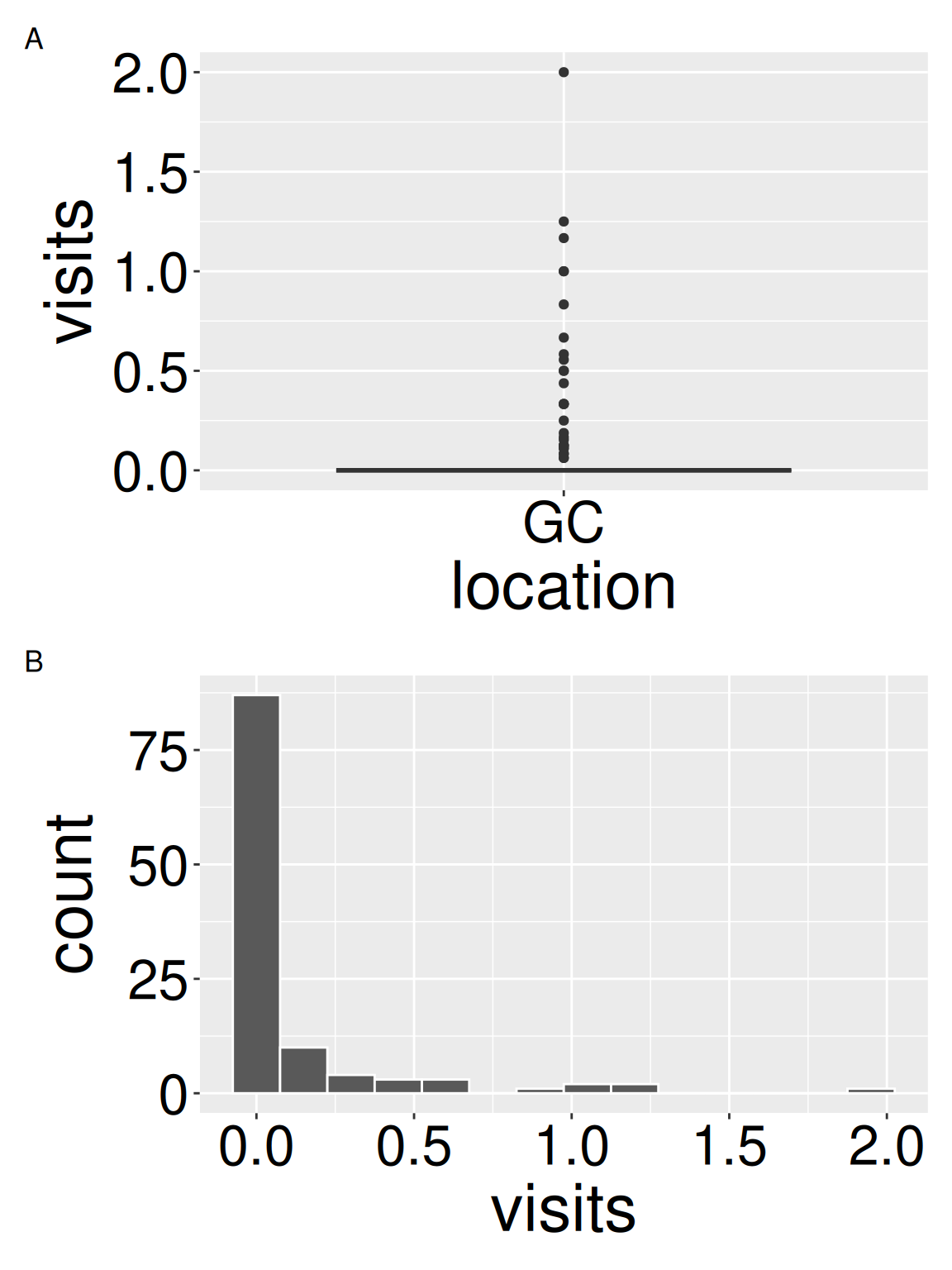
# The plots show highly right skewed data - most plants 
#   receive zero or few visits, some receive many
# I will continue with the standard run of summaries, 
#   but note, some are less appropriate for this shape

###--------------------------
### Data summaries

## Summarizing center
gc_visits |>
  summarise(mean_visits   = mean(visits),                # Mean
            median_visits = median(visits))              # Median

## Summarizing variability
gc_visits |>
  summarise(iqr_visits    = IQR(visits),                 # Interquartile range
            sd_visits     = sd(visits),                  # Standard deviation
            var_visits    = var(visits),                 # Variance
            coef_var_visits = sd(visits) / mean(visits)) # Coefficient of variation

Summarizing the average pollinator visits at GC

mean_visits	mode_visits	median_visits
0.1163	0	0

Summarizing variability in pollinator visits at GC

iqr_visits	sd_visits	var_visits	coef_var_visits
0	0.3055	0.0933	2.6269