Motivating scenario: In the previous section, we estimated slopes and quantified uncertainty around those estimates. But a skeptic might reasonably ask: could this association have been generated by chance? In this section, we introduce three approaches for testing the null hypothesis that the slope equals zero.
Learning goals: By the end of this section, you should be able to:
State the null hypothesis for a regression slope and explain what it means biologically.
Calculate and interpret a t-statistic and p-value for the slope of a linear regression.
Explain why the default p-value for an intercept is rarely interesting.
Use an ANOVA framework to partition variation into model and error sums of squares.
Calculate and interpret \(R^2\) as the proportion of variation in the response explained by the model.
Use a permutation test to generate a null distribution for a regression slope.
We have found slightly more than a half percentage point increase in percentage of seeds that are hybrid for each \(1\text{ mm}^2\) increase in petal area, and quantified uncertainty about this estimate. We also know that this relationship could have arisen by sampling error from a population in which no such relationship existed. Now we ask:
Can the observed relationship between petal area and proportion hybrid seed be easily attributed to sampling error?
We will go about this in three ways:
Reassuringly we will see that the t- and F- based analyses result in the exact same p-value, as seen previously.
Using the tools of the t-distribution to test if the slope is significantly different from zero.
Using the ANOVA framework to see if the variation attributable to the model exceeds that attributable to error.
Using permutation to see if the observed slope stands out from the distribution of slopes generated by random shuffling.
A t-based approach for NHST of linear regression
Does the intercept differ from zero?
Who cares that question is dumb. I will not calculate it for the intercept because its f$^&!ng stupid. HINT: It’s a t-distribution and the so-called null is 0.
Does the slope differ from zero?
We will first use a t-based approach to test the null of a slope of zero. Remember the steps of a t-based test
Calculate t as the distance, in standard errors, between our estimate and the null.
Find the p-value as the area in both tails of the t-distribution that is as extreme as, or more extreme than, the observed t-value. Because t is symmetric we usually take the absolute value of t and multiply the area on right tail by two to find the total area.
Reject the null if p < 0.05.
In the equation for \(SE_b\):
\(s_e\) is the standard deviation in residuals.
\(s_x\) is the standard deviation in the explanatory variable.
\(n\) is the sample size.
Because the null hypothesis says that the slope equals zero, the t-statistic is:
\[t = \frac{b - 0}{SE_b} = \frac{b}{SE_b}\]
As we saw earlier, the standard error of the slope is:
\[ SE_b = \frac{s_e / s_x}{\sqrt{n - 2}}\] Recalling that a linear regression with one explanatory variable has \(n-2\) degrees of freedom, we’re ready to go and calculate these values ourselves:
This p-value means that, if the true slope were zero, about 0.036% of repeated samples would generate a slope as far from zero as, or farther from zero than, the one we observed. So we reject the null hypothesis and conclude that petal area is associated with proportion hybrid seed in this dataset.
Interpreting R’s output
Of course, we don’t need to do these calculations, R does them for us. We can see this from either the summary() function in base R or broom’s tidy() function. Today we’ll do the latter, as tidy() returns less clutter than summary().
tidy(hybrid_lm)
term
estimate
std.error
statistic
p.value
(Intercept)
-0.20783
0.09947
-2.08950
0.03918
petal_area_mm
0.00574
0.00155
3.69085
0.00036
Recall, that the intercept is a part of our model that is essential for making predictions, but the null hypothesis of a value of zero is absurd. So I ignore everything except the estimate for the (Intercept).
The second row, with term petal_area_mm describes the slope. The tidy output provides its estimate, uncertainty (standard error), statistic (t-value), and the p-value! Reassuringly these results are the same as ours!
Does the model explain more variation than we would expect under the null?
Code for a the variance decomposition plot in the margin.
library(patchwork)a <-ggplot(mutate(gc_rils, mean_hyb =mean(prop_hybrid)) , aes(x = petal_area_mm, y = prop_hybrid)) +geom_point(alpha = .8, size =2) +geom_hline(aes(yintercept = mean_hyb)) +geom_segment(aes(xend = petal_area_mm, yend = mean_hyb), color ="black", alpha = .5) +labs(title ="Total deviation", y ="Prop hybrid", x ="Petal area (mm^2)")+theme(axis.text =element_text(size =22),axis.title =element_text(size =25),plot.title =element_text(size =28))b <-ggplot(mutate(augment(hybrid_lm), mean_hyb =mean(prop_hybrid)), aes(x = petal_area_mm, y = prop_hybrid)) +geom_point(alpha = .8, size =2) +geom_hline(aes(yintercept = mean_hyb)) +geom_segment(aes(xend = petal_area_mm, y = .fitted, yend = mean_hyb), color ="black", alpha = .5) +geom_line(aes(y = .fitted), color ="blue") +labs(title ="Model deviation", y ="Prop hybrid", x ="Petal area (mm^2)")+theme(axis.text =element_text(size =22),axis.title =element_text(size =25),plot.title =element_text(size =28))c <-ggplot(augment(hybrid_lm), aes(x = petal_area_mm, y = prop_hybrid)) +geom_point(alpha = .8, size =2) +geom_segment(aes(xend = petal_area_mm, yend = .fitted), color ="black", alpha = .5) +geom_line(aes(y = .fitted), color ="blue") +labs(title ="Error deviation", y ="Prop hybrid", x ="Petal area (mm^2)")+theme(axis.text =element_text(size =22),axis.title =element_text(size =25),plot.title =element_text(size =28))a/b/c +plot_annotation(tag_levels ="A",) +plot_layout(axis_titles ="collect") &theme(plot.tag =element_text(size =25))
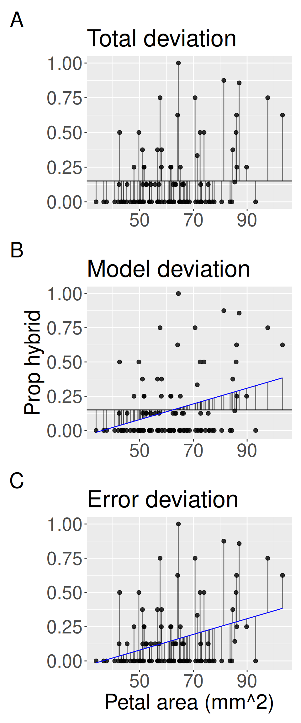
Figure 1: An ANOVA framework for linear regression.
A) shows the difference between each observation, \(Y_i\), and the mean \((\overline{Y})\) which is the basis for calculating the total sum of squares \((SS_{total})\).
B) shows the difference between each predicted value \((\widehat{Y_i})\) and the mean \((\overline{Y})\) which is the basis for calculating the model sum of squares \((SS_{model})\).
C) shows the difference between each observation \((Y_i)\) and its predicted value \((\widehat{Y_i})\), which is used to calculate the error sum of squares \((SS_{error})\).
We can also test the null using the variance-partitioning perspective of ANOVA (see previous chapters on ANOVA with two or more groups). Although the calculations for model and error sums of squares may initially look different than what we have done in the categorical ANOVA, they are conceptually identical (Figure 1).
SS_model is the sum of squared differences between predictions from the model and the global mean: \(SS_\text{model} = \sum(\widehat{Y_i} - \bar{Y})^2\).
SS_error is the sum of squared residuals: \(SS_\text{error} = \sum e_i^2 = \sum(Y_i - \widehat{Y_i})^2\).
The code below uses the output of broom’s augment() function to conduct an ANOVA-based test ot the null model. To do so it calculates:
SS_model as \(SS_\text{model} = \sum{(\hat{y_i} - \bar{y})^2 }\).
SS_error as \(SS_\text{error} = \sum e_i^2 = \sum(Y_i - \widehat{Y_i})^2\).
DF_model as the number of parameters to describe the slope (1).
DF_error as the number of data points “free to vary”. I.e. the sample size minus two (i.e. the two model parameters – slope and intercept).
MS_model as \(MS_\text{model} = SS_\text{model} / DF_\text{model}\).
MS_error as \(MS_\text{error} = SS_\text{error} / DF_\text{error}\).
F as \(F = MS_\text{model}/MS_\text{error}\).
p as the area more extreme than the observed F. This requires MS_model and MS_error. Because F must be positive, we only look at the right tail of its distribution and do not multiply by two to find p.
The p-values from the ANOVA and t-based approaches match! For a test of one slope in the same linear model, this happens because \(F = t^2\). This always makes me feel good about the world.
We can also find the proportion of variance explained by the model (\(R^2\)) as:
I’m always amazed that this equals the squared correlation coefficient: gc_rils |> summarise(r2 = cor(prop_hybrid , petal_area_mm)^2): 0.119.
R’s anova() table
Of course you can save yourself these calculations by just using base R’s anova() function. This will make you a nice ANOVA table:
anova(hybrid_lm)
Analysis of Variance Table

Response: prop_hybrid
               Df Sum Sq Mean Sq F value    Pr(>F)
petal_area_mm   1 0.6870 0.68700  13.622 0.0003625 ***
Residuals     101 5.0936 0.05043
---
Signif. codes:  0 '***' 0.001 '**' 0.01 '*' 0.05 '.' 0.1 ' ' 1
You can also pass this to broom’s tidy() function to make it easier to deal with in R:
anova(hybrid_lm) |>tidy()
term
df
sumsq
meansq
statistic
p.value
petal_area_mm
1
0.68700
0.68700
13.62238
0.00036
Residuals
101
5.09359
0.05043
NA
NA
Permutation based NHST
Because our data do not perfectly match assumptions of the linear regression (see prior section), we want to make sure this p-value is not fooling us. A simple way to do this is by a permutation test. As you may recall from the chapter on permutation this amounts to generating a null distribution by shuffling the association between explanatory and response values:
Our p-value from permutation is essentially identical to those above. This reassures us that our rejection of the null of no relationship between petal area and proportion hybrid seeds is not attributable to the deviation of our data from the linearity and equal variance assumptions of a linear model.
Together, these three approaches tell the same story. The observed relationship between petal area and proportion hybrid seed is much stronger than we would expect if there were no association between the variables. The t-test says the slope is large relative to its standard error, the ANOVA says the model explains much more variation than expected relative to residual error, and the permutation test shows that slopes this extreme are rare when we shuffle away the association.