• 20. Multiple regression summary

Links to: Summary. Chatbot tutor. Questions. Glossary. R functions. R packages. More resources.

Chapter summary

Multiple regression lets us model a response variable as a function of several explanatory variables at once. In additive models - like those in this chapter - we make predictions by adding up the contribution of each explanatory variable. With multiple regression, we ask if an explanatory variable is associated with the response after adjusting for other variables in the model. But don’t be fooled this adjustment is just that, an adjustment, and not a proper scientific control.

Chatbot tutor

Please interact with this custom chatbot (ChatGPT, or Gemini). I have made it to help you with this chapter. I suggest interacting with at least ten back-and-forths to ramp up and then stopping when you feel like you got what you needed from it.

Practice Questions

Try these questions! By using the R environment you can work without leaving this “book”. I even pre-loaded the packages you need.

Setup

To see if you can transfer these ideas beyond the Clarkia example, let’s use iris. Suppose we want to model petal length as a function of sepal length and species.


Call:
lm(formula = Petal.Length ~ Sepal.Length + Species, data = iris)

Coefficients:
      (Intercept)       Sepal.Length  Speciesversicolor   Speciesvirginica  
          -1.7023             0.6321             2.2101             3.0900

Q1) The model includes .

Q2) The coefficient for Sepal.Length describes the expected change in Petal.Length for a one cm increase in Sepal.Length,

Without accounting for species. After controlling for species After adjusting for species and petal width. Only for setosa plants. After adjusting for species.

Q3) The coefficient for Speciesversicolor compares versicolor petal length to

The average petal length of the other two Iris species. Setosa petal length, without accounting for sepal length. Virginica petal length, after adjusting for sepal length. Setosa petal length, after adjusting for sepal length. The extra change in petal length per 1 cm sepal length for versicolor compared with setosa.

Q4) It is better to say this model “adjusts for species” rather than “controls for species” because

Species is a categorical variable. The model cannot include species. Species has more than two levels. Species was not experimentally manipulated — whatever that would mean.

Plots should match models

Here are two ways of plotting petal length as a function of sepal length and species.

honestlm: use honest_lm() for guarded linear model summaries, or as_honest_lm(lm(...)) for existing lm objects.

`geom_smooth()` using formula = 'y ~ x'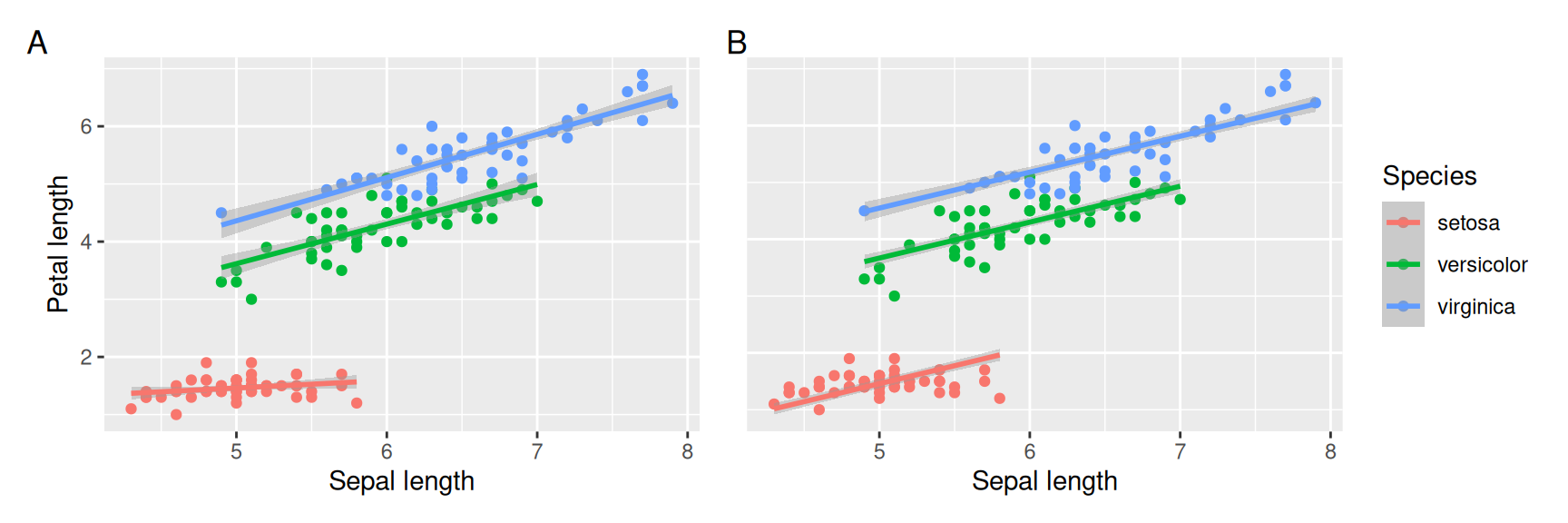

Scatterplot of iris petal length against sepal length, colored by species. Fitted lines are shown for each species with the lines being somewhat different in A (different slopes), and B (same slopes). — Figure 1: Petal length as a function of sepal length and species in iris. The two plots show the same data but with different models.

Q5) Which plot in Figure 1 best corresponds to the model, Petal.Length ~ Sepal.Length + Species?

A because each species gets its own slope. A because the lines minimize the sum of squared residuals separately for each species. B because all species share the same slope. Trick question, this is an opinion, not a fact.

Q6) Which function was used to add best fit lines in Figure 1 B?

Coefficient p-values are not always the tests we want

Here is the usual summary() output:

summary(iris_model)


Call:
lm(formula = Petal.Length ~ Sepal.Length + Species, data = iris)

Residuals:
     Min       1Q   Median       3Q      Max 
-0.76390 -0.17875  0.00716  0.17461  0.79954 

Coefficients:
                  Estimate Std. Error t value Pr(>|t|)    
(Intercept)       -1.70234    0.23013  -7.397 1.01e-11 ***
Sepal.Length       0.63211    0.04527  13.962  < 2e-16 ***
Speciesversicolor  2.21014    0.07047  31.362  < 2e-16 ***
Speciesvirginica   3.09000    0.09123  33.870  < 2e-16 ***
---
Signif. codes:  0 '***' 0.001 '**' 0.01 '*' 0.05 '.' 0.1 ' ' 1

Residual standard error: 0.2826 on 146 degrees of freedom
Multiple R-squared:  0.9749,    Adjusted R-squared:  0.9744 
F-statistic:  1890 on 3 and 146 DF,  p-value: < 2.2e-16

Q7) Why should we avoid using these p-values as our main NHST approach for multiple regression in this chapter?

Because R calculated them incorrectly. Because they test individual coefficients, not necessarily whole model terms. Because p-values cannot be calculated for linear models. Because p-values are wrong. Use Bayesian approaches instead.

Q8) For the species term, summary() gives rows for Speciesversicolor and Speciesvirginica. These are

Comparisons to setosa, after adjusting for sepal length. A test of whether species is significant, after adjusting for sepal length. Post-hoc tests to see which species matter, after adjusting for sepal length.

Instead, for additive multiple regression models, we use Type II sums of squares with car::Anova():

car::Anova(iris_model, type = "II")

Anova Table (Type II tests)

Response: Petal.Length
             Sum Sq  Df F value    Pr(>F)    
Sepal.Length 15.565   1  194.95 < 2.2e-16 ***
Species      99.802   2  624.99 < 2.2e-16 ***
Residuals    11.657 146                      
---
Signif. codes:  0 '***' 0.001 '**' 0.01 '*' 0.05 '.' 0.1 ' ' 1

Q9) The car::Anova() table above is useful because it tests

Only the intercept. Only the first term in the model. Model terms after accounting for the other terms in the additive model. Whether the residuals are normal.

Q10) Base R’s anova(iris_model) is inappropriate here because it uses

Type I, sequential sums of squares. Type II sums of squares. Post-hoc pairwise comparisons. Standardized coefficients.

Q11) If a categorical predictor with more than two levels is significant, the next natural question is often

What is the intercept p-value? Which levels differ from which other levels? Can I remove the response variable? Can I ignore the model assumptions?

Post-hoc tests and adjusted means

species_means <- emmeans::emmeans(iris_model, ~ Species)
species_means

 Species    emmean     SE  df lower.CL upper.CL
 setosa       1.99 0.0551 146     1.88     2.10
 versicolor   4.20 0.0402 146     4.12     4.28
 virginica    5.08 0.0523 146     4.98     5.18

Confidence level used: 0.95

emmeans::contrast(species_means, method = "pairwise", adjust = "tukey")

 contrast               estimate     SE  df t.ratio p.value
 setosa - versicolor       -2.21 0.0705 146 -31.362 <0.0001
 setosa - virginica        -3.09 0.0912 146 -33.870 <0.0001
 versicolor - virginica    -0.88 0.0638 146 -13.800 <0.0001

P value adjustment: tukey method for comparing a family of 3 estimates

Q12) The estimated means above are

Raw species means. Model-adjusted means. Residuals. Variance inflation factors.

Q13) The pairwise contrasts above ask which

Species differ from one another after adjusting for sepal length. Individual iris plants are outliers after adjusting for sepal length.. Variables are normally distributed. Terms should be entered first in the model.

Effect sizes and assumptions

Q14) Why is it hard to compare the raw coefficient for Sepal.Length to the raw coefficient for Speciesversicolor?

Because they describe different kinds of comparisons. Because one is a response variable and the other is not. Because categorical variables cannot be included in regression. Because coefficients are always unitless.

Q15) What information is conveyed by partial \(R^2\) that we cannot get from looking at model coefficients?

The direction of the association between a predictor and the response. The expected change in the response for a one-unit change in a predictor. How much variation in the response is associated with a term after accounting for the others. Which variable causes the resposne.

📊 Glossary of Terms

📚 1. Model Concepts

Multiple regression: A linear model with more than one explanatory variable.
Additive model: A model in which we add the contributions of explanatory variables, without interactions.
Conditional association: The association between a focal explanatory variable and the response after adjusting for other variables in the model.
Statistical adjustment: Including a variable in a model to account for its association with the response and/or other predictors. This is not experimental control.

📏 2. Model Evaluation

Type I sums of squares: Sequential sums of squares. Results can depend on the order of terms in the formula.
Type II sums of squares: Sums of squares for a term after accounting for other terms in an additive model.
Partial \(R^2\): A term-level effect size describing how much residual variation is reduced by adding a focal term.
VIF: Variance inflation factor; a measure of how much uncertainty in a coefficient is inflated by correlations among predictors.
Model-adjusted mean: A predicted mean for a group after accounting for other variables in the model.

🛠️ Key R Functions

Building and interpreting models

lm(y ~ x1 + x2 + group, data = data) fits an additive multiple regression.
honest_lm(y ~ x1 + x2 + group, data = data) fits an additive multiple regression with guardrails.
broom::tidy(model, conf.int = TRUE) creates a coefficient table with confidence intervals.
broom::augment(model) adds fitted values and residuals to the data.
ggfortify::autoplot(model) makes standard diagnostic plots for a fitted model.

Significance, effect sizes, and uncertainty

car::Anova(model, type = "II") gives Type II term-level tests.
emmeans::emmeans(model, ~ group) estimates model-adjusted means.
emmeans::contrast(..., method = "pairwise", adjust = "tukey") runs post-hoc tests.
car::vif(model) calculates variance inflation factors.
honestlm::partial_r2(model) calculates partial \(R^2\) and Cohen’s \(f^2\).
honestlm::av_transform() helps make added variable plots.
modelbased::estimate_means(model, by = "group") estimates model-adjusted means.
modelbased::estimate_slopes(model, trend = "x") estimates model-based slopes.
parameters::standardize_parameters(model) reports standardized coefficients.

Model-matching plots

honestlm::geom_lm_smooth() plots additive linear-model smooths.
honestlm::stat_lm_means() plots additive model-based means.

R Packages Introduced

car: Provides tools for regression diagnostics and term-level tests, including Anova() for Type II sums of squares and vif() for multicollinearity.
emmeans: Estimates model-adjusted means and compares them with post-hoc contrasts.
honestlm: Provides helper functions for plotting additive linear models and calculating partial \(R^2\).
broom: Converts model output into tidy data frames with tidy() and augment().
modelbased: Estimates model-based means, slopes, predictions, and contrasts.
parameters: Summarizes and standardizes model parameters.
ggfortify: Makes diagnostic plots for models with autoplot().

Additional resources

Blog posts:

Regression fire and dangerous things. A blog post by Richard McElreath that explains the problem with the “causal salad” of multiple regression.
How to break regression. A nice explanation with r based simulation code about how what you put in your model matters.
Why Adjusted Regression Coefficients Are Less Descriptive Than They Look. I nice blogpost with interactive apps which highlight how coeffcieints from a multiple regression depend on other variables in the model.

Videos

Statistics 101: Multiple regression playlist, ANCOVA playlist.

Book Chapters

ModernDive: Multiple Regression: Another tidyverse focused overview of multiple regression