Optional: Simulating from the Normal Distribution

Motivating scenario: We want to learn how to use R to generate random samples from a normal distribution to build intuition and verify its theoretical properties.

Learning goals: By the end of this chapter you should be able to:

1. Use R’s rnorm() function to simulate random draws from any normal distribution.
2. Simulate a sampling distribution of the mean of a normally distributed random variable.
3. Use rnorm()’s output to verify a theoretical properties of the normal distribution.

---

Simulating from Normal Distributions in R

In the previous section, we used a web app to calculate probabilities from a normal distribution. Here, we’ll take a different approach: simulation. We’ll use R’s rnorm() function to generate our own random data. This approach both builds intuition for the sampling process and allows us to double-check our math.

Simple Simulation with rnorm()

We previously saw that about 68% of a normal distribution falls within one standard deviation of the mean. We can validate this for ourselves by a simple simulation, using our log-transformed petal area (\(X \sim \mathcal{N}(1.78,\,0.01)\)) as an example. To do so

• We first simulate the data with rnorm() (see simulated data in the margin).
  
• We then find the proportion of draws within one standard deviation (i.e. greater than 1.68 and less than 1.88, code and answer below:)

normal_sim <- tibble(x = rnorm(mean = 1.78, sd = 0.1, n = 1000) )

normal_sim |>
  mutate(within_sd = x > 1.68 & x < 1.88) |>
  summarise( prop_within_sd = mean(within_sd))

# A tibble: 1 × 1
  prop_within_sd
           <dbl>
1           0.67

This is close to our mathematical result, but sampling variability leaves this a bit off our precise expectation of 0.6826895.

rnorm() (and all _norm() functions) defaults to the standard normal, so rnorm(n = 10) generate a sample of ten observations from a normal distirbution.

Multiple samples from a normal

We know by now that the standard error is the standard deviation of the sampling distribution. I briefly informed you that for the normal the mathematical formula for the standard error of the mean is:

\[\sigma_\bar{x} = \sigma/\sqrt{n}\text{ where: }\]

• \(\sigma = \sqrt{\frac{\Sigma{(x_i-\mu)^2}}{n}}\).
  
• \(n\) is the sample size.

Let’s convince ourselves of this by simulation and then make sure that \(\approx 68\%\) of sample means, \(\bar{x}\) are within one SE of the population mean \(\mu\).

To do so we will set up a scenario in which our simulation results are “grouped”. Summarizing each sample with the mean generates a sampling distribution.

Note for the simulation below:

• We simulated from the standard normal distribution (\(X \sim \mathcal{N}(0,\,1)\)).
  
• We simulated one hundred thousand samples each of size nine.

mu               <- 0 
sigma            <- 1
sample_size      <- 9 
n_samples        <- 100000

normal_sampling_sim <- tibble(
  x = rnorm(mean = mu, sd = sigma, n = sample_size * n_samples),
  group = rep(1:n_samples, each = sample_size)
)

sample_means <- normal_sampling_sim |>
  group_by(group)   |>
  summarise(mean_x = mean(x))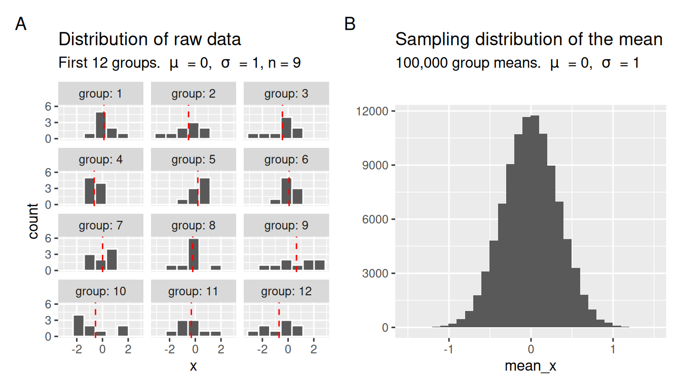

Figure 1: Simulating many samples of size 9 from a population with μ=0 and σ=1. A. The first 12 random samples. Note the variability in the shapes of the histograms and the sample means (red dashed lines). B. The sampling distribution of the mean, constructed from 100,000 sample means. Note that the spread of of data in each sample (A), exceeds the spread of sample means in B.

We can calculate the standard deviation of the sample means in Figure 1 as shown in the margin. You can see that the standard deviation of the sampling distribution of the standard normal with a sample size of 9 is approximately \(1/3\), which reassuringly is the standard deviation (\(\sigma = 1\)) divided by the square root of the sample size, \(\sqrt{n} = \sqrt{9} =3\).

sample_means |> 
  summarise(se = sd(mean_x))

# A tibble: 1 × 1
     se
  <dbl>
1 0.335

Multiple samples from a normal within a range

We expect, for example, \(\approx 68\%\) of draws from the normal to be within one standard deviation of the mean. We similarly expect \(\approx 68\%\) of sample means to be within one standard error of the population mean (i.e. between \(\mu-\frac{\sigma}{\sqrt{n}}\) and \(\mu+\frac{\sigma}{\sqrt{n}}\)). We can confirm this was true of our simulation as follows:

se    <- sigma / sqrt(sample_size)

sample_means |> 
  mutate(within_one_se     = mean_x > mu - se &    mean_x < mu + se) |>
  summarise(prop_within_se = mean(within_one_se))

# A tibble: 1 × 1
  prop_within_se
           <dbl>
1          0.681