• 21. Interactions summary

Links to: Summary. Questions. Glossary. R functions. R packages. More resources.

---

Chapter summary

Sometimes the impact of changing one variable depends on the value of another. Such statistical interactions can both illuminate biological processes and complicate stiatical analyses and interpretation. This chapter explains the best practices when modelling statistical interactions. I then show how we can think of an interaction of a variable with itself as a polynomial regression. This section serves to show that “linear models” can fit curved data.

Practice Questions

Try these questions using the penguins data.

Setup

penguin_additive_model    <- lm(body_mass ~ sex + species, data = penguins)
penguin_interaction_model <- lm(body_mass ~ sex + species + sex:species, data = penguins)

Q1) The sex:species interaction in penguin_interaction_model asks whether

Male penguins are heavier than female penguins. Penguin species differ in average body mass. The male-female difference in body mass differs among species. The proportion of males and females differs among species.

---

Consider the coefficients from the models

Additive model

# **Additive model**
coef(penguin_additive_model)

(Intercept)	sexmale	speciesChinstrap	speciesGentoo
3372	668	27	1378

Q2) For the additive model, predict the mean body mass of a Female Gentoo penguin: \(\widehat{Y}_{\text{female Gentoo}}\) =

Q3) For the additive model, predict the mean body mass of a Male Gentoo penguin: \(\widehat{Y}_{\text{male Gentoo}}\) =

---

Interaction model

(Intercept)	sexmale	speciesChinstrap	speciesGentoo	sexmale:speciesChinstrap	sexmale:speciesGentoo
3369	675	158	1311	-263	130

Q4) For the interaction model, predict the mean body mass of a Female Gentoo penguin: \(\widehat{Y}_{\text{female Gentoo}}\) =

Q5) For the interaction model, predict the mean body mass of a Male Gentoo penguin: \(\widehat{Y}_{\text{male Gentoo}}\) =

---

Visualizing the interaction

Figure 1: Body mass by sex and species in the penguins data. Points show observed penguins. Large points show group means.

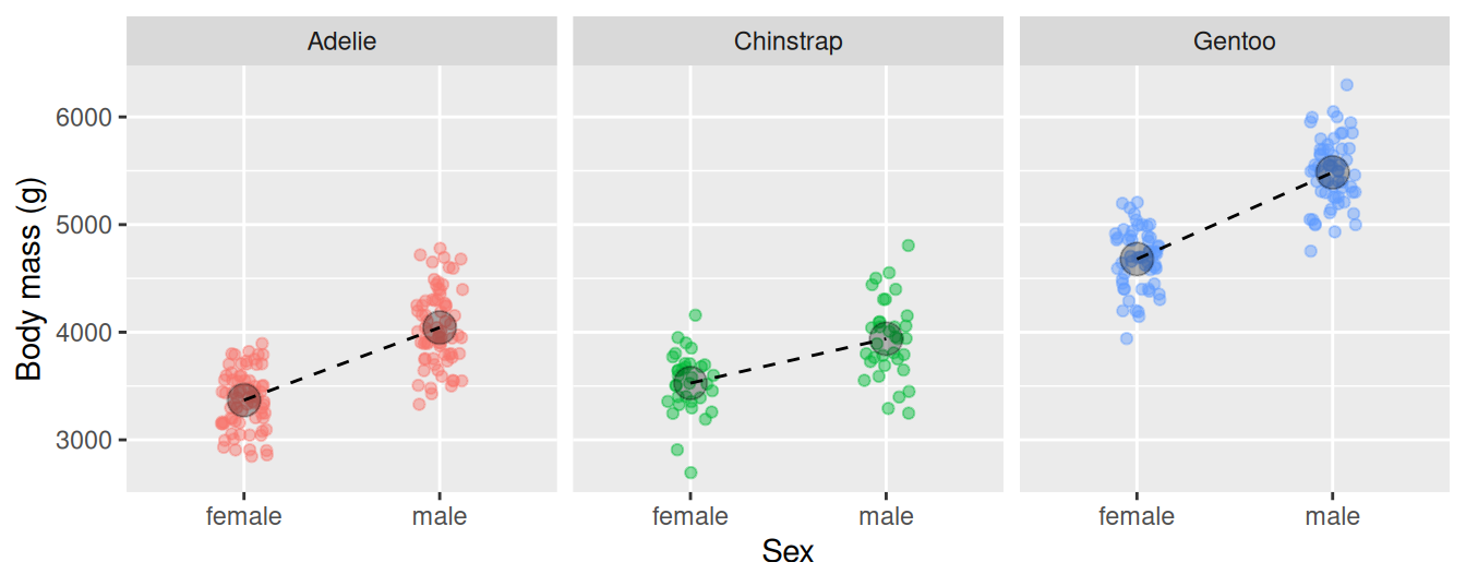
Q6) Which aspect of Figure 1 suggests an interaction between sex and species?

That body mass differs by species. That body mass differs by sex, i.e. the line connecting male and female means has a non-zero slope. That the line connecting male and female means is steeper for Gentoo penguins than for Adelie and Chinstrap penguins. Such plots do not convey information about interactions.

---

Testing the interaction

library(car)
Anova(penguin_interaction_model, type = "II")

Anova Table (Type II tests)

Response: body_mass
               Sum Sq  Df F value    Pr(>F)    
sex          37090262   1 387.460 < 2.2e-16 ***
species     143401584   2 749.016 < 2.2e-16 ***
sex:species   1676557   2   8.757 0.0001973 ***
Residuals    31302628 327                      
---
Signif. codes:  0 '***' 0.001 '**' 0.01 '*' 0.05 '.' 0.1 ' ' 1

Q7) Why did we use car::Anova() rather than base R’s anova() here?

Because base Rs anova() uses sequential Type I sums of squares, so results can depend on the order of terms in the model. Because base R cannot fit models with interactions. Because anova() assumes that residuals are normally distributed. Because car::Anova() proves that the interaction is causal.

Q8) The small p-value for sex:species means we reject the null that

Male and female penguins have the same average body mass. All penguin species have the same average body mass. Sex and species are independent. The sex difference in body-mass is identical across species.

---

Consider summary() output

summary(penguin_interaction_model)

Call:
lm(formula = body_mass ~ sex + species + sex:species, data = penguins)

Residuals:
    Min      1Q  Median      3Q     Max 
-827.21 -213.97   11.03  206.51  861.03 

Coefficients:
                         Estimate Std. Error t value Pr(>|t|)    
(Intercept)               3368.84      36.21  93.030  < 2e-16 ***
sexmale                    674.66      51.21  13.174  < 2e-16 ***
speciesChinstrap           158.37      64.24   2.465  0.01420 *  
speciesGentoo             1310.91      54.42  24.088  < 2e-16 ***
sexmale:speciesChinstrap  -262.89      90.85  -2.894  0.00406 ** 
sexmale:speciesGentoo      130.44      76.44   1.706  0.08886 .  
---
Signif. codes:  0 '***' 0.001 '**' 0.01 '*' 0.05 '.' 0.1 ' ' 1

Residual standard error: 309.4 on 327 degrees of freedom
Multiple R-squared:  0.8546,    Adjusted R-squared:  0.8524 
F-statistic: 384.3 on 5 and 327 DF,  p-value: < 2.2e-16

Q9) Consider the (Intercept) p-value.

• Q9.A) This tests the null hypothesis that
  The mean body mass of female Adelie penguins is zero. The mean body mass of all penguins is zero. Sex has no association with body mass. Species has no association with body mass.
• Q9.B) This test is silly because
  Female Adelie penguins are not the reference group. We already know penguins do not have an average body mass of zero grams. Intercepts cannot be estimated in models with interactions. A small intercept p-value means the model is wrong.
  .

Q10) Why should we be cautious about interpreting the speciesChinstrap p-value from summary(penguin_interaction_model)? NOTE: Find all correct answers

It is only one reference-level comparison, not a test of the whole species term. Main effects require extra care when interactions are in the model. It does not account for the fact that we might make multiple species comparisons. Because Chinstrap penguins were randomly assigned to species.

All but the final answer are correct.

---

emmeans output

Consider the following output from emmeans() (I know we used model based but i like the warnings emmeans provides).

emmeans(penguin_interaction_model, pairwise ~ sex)

NOTE: Results may be misleading due to involvement in interactions

 contrast      estimate   SE  df t.ratio p.value
 female - male     -631 35.7 327 -17.659 <0.0001

Results are averaged over the levels of: species 

emmeans(penguin_interaction_model, pairwise ~ species)

NOTE: Results may be misleading due to involvement in interactions

 contrast           estimate   SE  df t.ratio p.value
 Adelie - Chinstrap    -26.9 45.4 327  -0.593  0.8241
 Adelie - Gentoo     -1376.1 38.2 327 -36.007 <0.0001
 Chinstrap - Gentoo  -1349.2 47.0 327 -28.682 <0.0001

Results are averaged over the levels of: sex 
P value adjustment: tukey method for comparing a family of 3 estimates 

Q11) Why does emmeans() warn that the sex comparison “may be misleading due to involvement in interactions”?

Because sex cannot be included in a model with species. Because the sex effect is not statistically significant. Because the estimated sex difference is averaged over species, even though the sex difference differs somewhat among species. Because emmeans() cannot calculate contrasts for categorical variables.

Q12) With the caveat above in mind, is it reasonable to say that males are heavier than females?

No, because any interaction makes main effects meaningless. Yes, but we should also say that the size of the male-female difference varies among species. Yes, and the interaction means the male-female difference is exactly the same in every species. No, because female Gentoo penguins have a greater body mass than male chinstrap penguins.

Q13) The female - male contrast from emmeans(penguin_interaction_model, pairwise ~ sex) estimates

The sex difference for reference group (Adelie penguins) only. The sex difference averaged over species. The sex:species interaction term.

Q16) Why does the non-significant Adelie - Chinstrap contrast from emmeans(…, pairwise ~ species) differ from the significant speciesChinstrap p-value in summary(penguin_interaction_model)? (NOTE: Find the two correct answers)

The emmeans() contrast compares Adelie and Chinstrap averaged over sex, while speciesChinstrap compares female Chinstrap to female Adelie. The emmeans() contrast tests sex, while speciesChinstrap tests body mass. The emmeans() p-value is adjusted by Tukey's method, while the speciesChinstrap p-value is not. They are the same test, so one of them must be wrong. Sampling error - these values are influence by chance.

Q17) Q) Which of the following are linear models?

Modeling blood glucose in lizards kept at warm vs. cool temperatures. Modeling algal growth as a function of nutrient concentration allowing for a hump or trough in this relationship. Modeling tadpole growth as a function of pond after adjusting for initial body size. Modelling the didferent effect of fertilizer on plant height in wet and dry soil. Modeling (log-transformed) metabolic rate as a function of (log-transformed) body mass. All of the above.

Glossary of Terms

• Statistical interaction: A pattern in a model where the association between one explanatory variable and the response depends on another explanatory variable.

• Biological interaction: A situation where two biological factors combine in a way that changes the outcome, such that their joint effect is not simply the sum of their separate effects.

• Interaction term: The part of a model that allows the effect of one explanatory variable to depend on another explanatory variable, such as sex:species or petal_area_mm:petal_color.

• Additive model: A model where explanatory variables contribute separately to the prediction. In an additive model, the model adds the effects of each predictor but does not let one predictor change the effect of another.

• Main effect: The association between one explanatory variable and the response, apart from any interaction terms. In models with interactions, main effects often require extra care.

• Partial R²: The proportion of remaining variation in the response associated with a model term after accounting for the other terms in the model.

• Polynomial regression: A regression model that includes powers of a predictor, such as x and x^2, to describe curved relationships.

• Quadratic term: A squared predictor, such as I(x^2), used to model curvature.

Key R Functions

• lm(y ~ x1 * x2, data = data) fits a model with the main effects of x1 and x2, plus their interaction.

• lm(y ~ x1 + x2 + x1:x2, data = data) fits the same interaction model, but writes the interaction term explicitly.

• : specifies an interaction term between predictors in a model formula.

• * expands to main effects plus their interaction. For example, x1 * x2 means x1 + x2 + x1:x2.

• I(x^2) tells R to include the squared value of x in a model formula.

• poly(x, degree = 2) includes polynomial terms for x, often used for quadratic or higher-order relationships.

• car::Anova(model, type = "II") gives Type II term-level tests.

• car::Anova(model, type = "III") gives Type III term-level tests, often used when interpreting models with interactions.

• emmeans::emmeans(model, pairwise ~ x) estimates marginal means and pairwise contrasts for x.

• emmeans::emmeans(model, pairwise ~ x | z) estimates pairwise contrasts for x separately within levels of z.

• emmeans::contrast(...) tests specific contrasts among estimated means.

• modelbased::estimate_means(model, by = ...) estimates model-based means or predictions.

• modelbased::estimate_slopes(model, trend = ..., by = ...) estimates slopes within levels or values of another predictor.

• geom_smooth(method = "lm") plots fitted linear-model relationships, including separate fitted lines when data are grouped.

R Packages Introduced

• modelbased: Estimates model-based predictions, means, contrasts, and slopes. Useful here for turning interaction models into interpretable quantities.

• emmeans: Estimates marginal means and contrasts. Useful for comparing groups, especially when interactions make raw coefficients hard to read.

• honestlm: Provides helper functions for teaching and visualizing linear models, including interaction-friendly model plots and partial \(R^2\).

• car: Provides Anova(), which we use for Type II and Type III term-level tests.

Additional resources

• Interactions in factorial designs, by Carlisle Rainey.Describes why interactions are hard to estimate and why studies often have less power for interactions than for main effects, and has an accompanying R packge.

• You need 16 times the sample size to estimate an interaction than to estimate a main effect, explained, by Andrew Gelman.

• Interaction Effects: A brief introduction from Penn State’s Stat462 site. I like these guys.

• Interaction variables. A youtube video from Nathan Wozny

.