Motivating scenario: You ran a model with interactions, estimated parameters, and even evaluated significance. Now what? The results are hard to think about and explain. To understand the biology, I show you how to translate this model into meaningful predictions, estimates, and measures of explained variation.
Learning goals: By the end of this section, you should be able to:
Use model-based estimates to describe uncertainty in predicted means and slopes.
Use partial (R^2) to summarize how much additional variation is explained by an interaction.
Write a concise biological interpretation of these results.
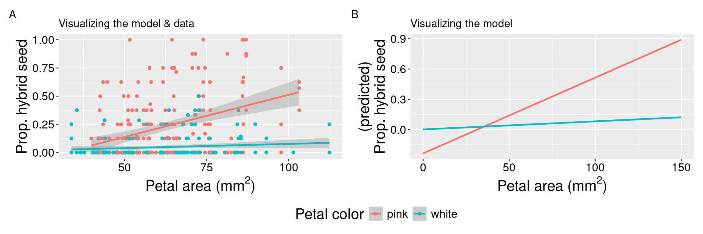
Figure 1: Observed and model-predicted relationships between petal area and the proportion of hybrid seed for pink- and white-petaled RILs. Panel A shows the data and the fitted model. Panel B extends the fitted lines to a petal area of zero to show what the model parameters are describing and how they can mislead us.
We modelled the proportion of hybrid seeds on a RIL as a function of petal area, petal color, and their interaction. If you recall there was some weirdness - the model returned a large and positive coefficient for petal_colorwhite, even though we found no region of our data in which the model predicted that white-petaled RILs would have a higher proportion of hybrid seeds than pink-petaled RILs (Figure 1 A).
We realized that this was because the coefficient of 0.2373 for petal_colorwhite describes the difference between its expected value at the intercept (i.e. petal_area_mm = 0, Figure 1 B) and that of the pink-petaled RILs. This prediction has no biological application, as no plants have petals of size zero \(mm^2\).
name
value
(Intercept)
-0.2356
petal_colorwhite
0.2373
petal_area_mm
0.0075
petal_colorwhite:petal_area_mm
-0.0067
Biological meaning from models
So, if we can’t get simple biological meaning from raw model coefficients, how can we make sense of our models? My best advice is to generate meaningful estimates of predicted means + uncertainty in them, for a few illustrative values of the explanatory variables.
Let’s start by doing this ourselves, by simply plugging in petal areas of 45 and 85 \(mm^2\) for white- and pink- petaled RILs into the model with interactions. I will also provide predictions from a linear model with no interactions for reference. Click the section below if you want to see this math:
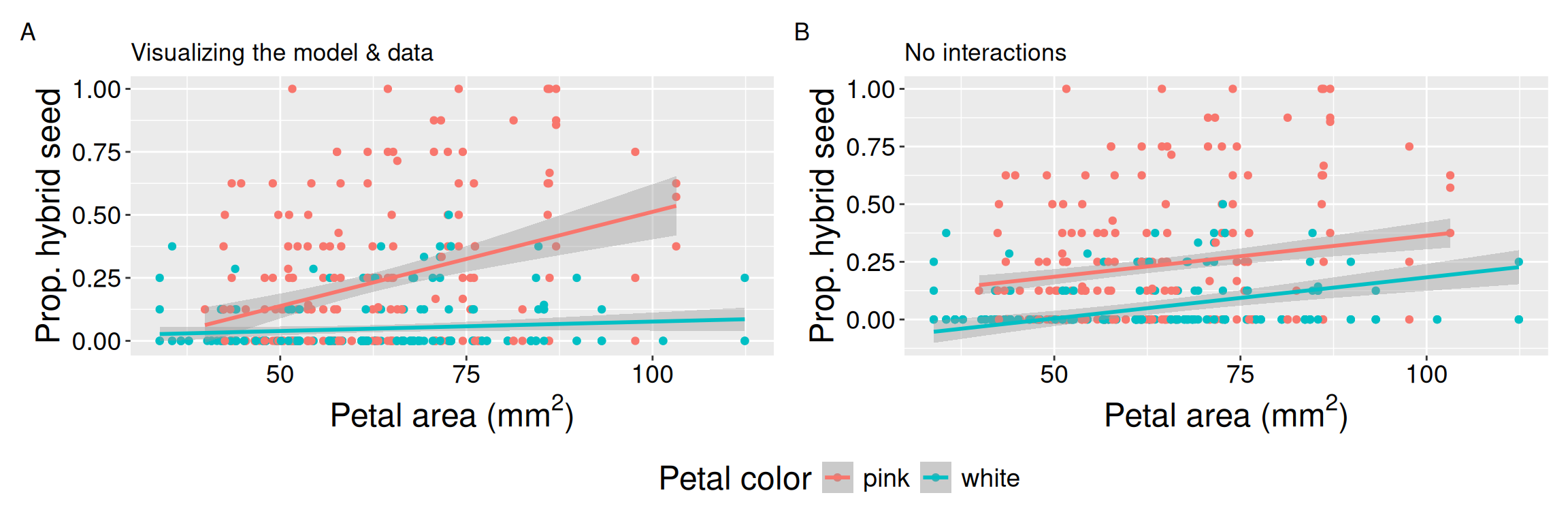
Figure 2: Predicted relationships between petal area and the proportion of hybrid seed under models with and without an interaction. Panel A shows the interaction model. Panel B shows the additive model.
In the interaction model, the predicted proportion of hybrid seed increases strongly with petal area among pink-petaled RILs but changes little among white-petaled RILs (Figure 2 A). So the predicted difference between colors is much larger at \(85 mm^2\) than at 45 \(mm^2\). Because the additive model predicts the same increase with petal area for both petal colors, the predicted difference between pink- and white-petaled RILs is constant across petal areas (Figure 2 B).
How much does the interaction explain?
\(R^2\), the proportion of variation explained is a standard summary of “effect size.” In the section on multiple regression, we saw that we could calculate partial \(R^2\) as:
\[R^2_\text{partial} = 1-\frac{SS_\text{error (full model)}}{SS_\text{error (model without focal predictor)}}\]
For an interaction model we do the same thing, first for a main effects model:
library(honestlm)lm(prop_hybrid ~ petal_color + petal_area_mm, data = rils)|>partial_r2()
We see that petal color and petal area “explain” 16% and 6% of the variance in the proportion of hybrid seeds on a RIL, respectively, after adjusting for the other variable.
And then for the interaction:
library(honestlm)lm(prop_hybrid ~ petal_color * petal_area_mm, data = rils)|>partial_r2()
# A tibble: 1 × 4
  term                         df partial_r2     f2
  <chr>                     <dbl>      <dbl>  <dbl>
1 petal_color:petal_area_mm     1     0.0579 0.0614
After adjusting for these main effects, the interaction between petal area and petal color explains 5% of the remaining variance in the proportion of hybrid seeds. Thus this interaction explains nearly as much variation in the proportion of hybrid seeds as petal area itself!!!
Describing uncertainty
Of course, no statistical description is complete without a measure of uncertainty. Again we can accomplish this with the emmeans or modelbased packages. Here I use estimate_means() function in the modelbased package, because I find it easier to code.
So to find uncertainty about the point estimates of the proportion of hybrid seeds for pink- and white-petaled RILs with petal area of 45 and 85 \(mm^2\), we type:
The two confidence intervals describe uncertainty in each slope. Note that they do not directly test the difference between slopes, as we do this by testing the interaction.
Writing up our results
Let’s try to synthesize these results into a brief “results” paragraph:
We tested the contribution of petal color, petal area and their interaction to the proportion of hybrid seeds on a RIL. Using Type II sums of squares, we found significant associations between the proportion of hybrid seeds and petal color (\(F_{1,398}\) = 80.23, p < 2.2e-16), petal area (\(F_{1,398}\) = 28.2, p < 2 e-7), and their interaction (\(F_{1,398}\) = 24.4, p < 2 e-6). This interaction reflects the sharp increase in the proportion of hybrid seed with petal area in pink-, but not white-petaled RILs (compare slopes of 0.0075 – 95% CI: {0.0054 : 0.0095} and 0.0007 – 95% CI: {-0.0010 : 0.0025}, respectively).