Motivating Scenario:
You are beginning to think about statistical models, and want to use something you understand well to ramp you up to more complex models.
Learning Goals: By the end of this subchapter, you should be able to:
Interpret residuals in a simple model.
Define and calculate residuals: the difference between observed values and model predictions.
Identify and estimate residuals from a plot.
Use R to explore and visualize residuals.
Use augment() to extract fitted values and residuals.
Calculate the sum of squared residuals and the residual standard deviation.
OPTIONAL: Understand that the mean minimizes the sum of squared residuals.
- And understand what the sentence above means.
Residuals
In a simple linear model with no predictors, the model predicts the same value for every observation: the mean. This means we predict the \(i^{th}\) individual’s value of the response variable to be \(\hat{y}_i = b_0\), where \(b_0\) is the mean.
Figure 1: The residual \(e_i\) is the difference between a data point and its value predicted from a model.
In reality, of course, observations rarely match prediction perfectly.
So for individual, \(i\), the observed value equals the predicted value plus the residual:
\[{y}_i = \hat{y}_i + e_i\]
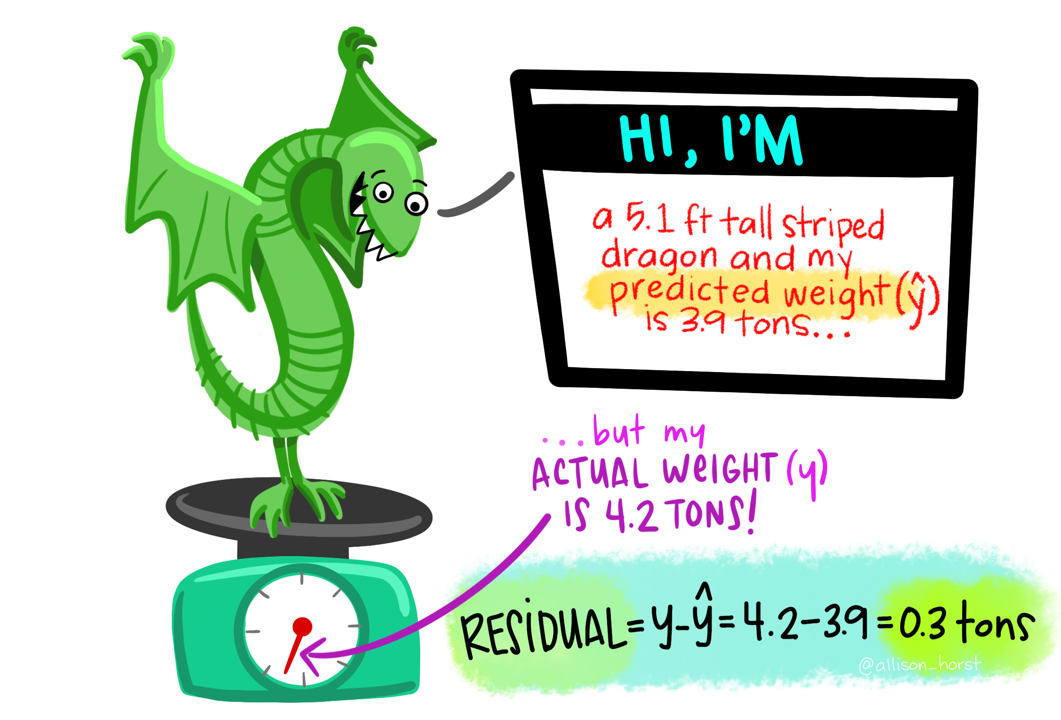
The residual, \(e_i\), is the difference between the observed and predicted value of the response variable in a given individual. With some rearrangement, we can restate the residual as follows:
\[e_i = {y}_i - \hat{y}_i\]
Positive residuals mean the observation is above the model prediction, while negative residuals mean it is below the model prediction.
Visualizing and Calculating Residuals
Worked example.
Take, for example, individual 14 (\(i = 14\), green point in the plot above), where five of eight (0.625) of its seeds are hybrids:
Its observed value, \(y_i\), is the proportion of its seeds that are hybrids, which is 0.625.
Its predicted value, \(\hat{y}_i\), is the proportion of all seeds that are hybrids (dashed red line), which is 0.151.
Its residual value, \(e_i = y_i - \hat{y}_i\), is the difference between the proportion of its seeds that are hybrids and proportion of all seeds that are hybrids, which is \(0.625 -0.151 = 0.474\). Scroll over the fourteenth data point in Figure 2 to verify this.
CHALLENGE: Fill in the blank. “The residual for individual 96 equals ___.”
Code
library(plotly)prop_hybrid_plot <- gc_rils |>filter(!is.na(prop_hybrid)) |>mutate(i =1:n(),e_i = prop_hybrid -mean(prop_hybrid),e_i =round(e_i, digits =3),y_hat_i =round(mean(prop_hybrid),digits =3),y_i =round(prop_hybrid, digits =3)) |>ggplot(aes(x = i, y = y_i, y_hat_i = y_hat_i, e_i = e_i, color = i%in%c(14,96)))+annotate(geom ="segment", x =14, xend=14,y = .151, yend =.625, size =2,lty =2, alpha = .4)+geom_point(size =4, alpha = .6)+scale_color_manual(values =c("black","darkgreen"))+geom_hline(yintercept =summarise(gc_rils,mean(prop_hybrid)) |>pull(),linetype ="dashed", color ="red", size =2)+labs(y ="Proportion hybrid", title ="This plot is interactive!! Hover over a point to see its residual")+theme(legend.position ="none")ggplotly(prop_hybrid_plot)
Figure 2: An interactive plot showing the proportion of hybrid seeds for eachClarkia xantiana subspecies parviflorarecombinant inbred line (RIL) planted at GC. Each point represents a line’s observed proportion hybrid seed, and the dashed red line shows the sample mean across all lines. Hovering over a point reveals its residual — the difference between the observed value and the mean. Individuals 14 and 96 are shown in green, examples to focus on. For further explanation, the dashed line connects individual 14’s observed proportion hybrid to the value predicted by the model.
Use augment() to show residuals (and more!)
You can use the augment() function in the broom package to see predictions and residuals. The code to the right uses this capability to calculate the sum of squared residuals, while the code below shows (some of) the output from augment().
library(broom)lm(prop_hybrid ~1, data = gc_rils) |>augment() |>select(prop_hybrid, .fitted, .resid)
Calculating \(\text{SS}_\text{residual}\) from augment() output
A basic summary of a model is how well it predicts each data point. One such summary is the Sum of Squared Residuals, \(\text{SS}_\text{residual}\). We will see soon that this plays a major role in evaluating and comparing linear models.
You can use the output of augment() to calculate the sum of squared residuals by taking residuals (from .resid), squaring them, and then summing them, as shown below:
library(broom)lm(prop_hybrid ~1, data = gc_rils) |>augment() |>mutate(sq_resid=.resid^2)|>summarise(SS=sum(sq_resid))
# A tibble: 1 × 1
     SS
  <dbl>
1  5.62
The standard deviation again?
“But we already had a section on the standard deviation. Why another section on this?”
You, probably.
We can now calculate the residual standard deviation, as \[s_\text{resid}=\sqrt{\frac{\text{SS}_\text{residual}}{n-1}} = \sqrt{\frac{\sum{e_i^2}}{n-1}}\]
Somewhat confusingly, the residual standard deviation is sometimes called the “residual standard error.”
lm(prop_hybrid ~1, data = gc_rils) |>augment() |>mutate(sq_resid=.resid^2)|>summarise(SS_resid =sum(sq_resid), n =n(),sd_resid =sqrt(SS_resid / (n -1)))
# A tibble: 1 × 3
  SS_resid     n sd_resid
     <dbl> <int>    <dbl>
1     5.62   101    0.237
R can calculate this for us by using the sigma() function on the linear model output:
lm(prop_hybrid ~1, data = gc_rils) |>sigma()
[1] 0.2371298
So there are numerous ways to use R calculate the residual standard deviation (aka residual standard error) – a classic description of how well the model fits the data.
Of course, because we have a model with only a mean at the moment the residual standard deviation is just the standard deviation: gc_rils |> summarise(sd(prop_hybrid)): 0.2371.
STOP HERE UNLESS YOU REALLY WANT MORE
OPTIONAL / ADVANCED
The mean minimizes \(\text{SS}_\text{residual}\)
You already know the formula for the mean. But let’s imagine you didn’t. What properties would you want a good summary of the center of the data to have? What criteria would you use to say one summary was the best? We have already discussed this at length, and concluded it depends on the shape of the data etc…
While you should consider the shape of our data when summarizing it, a common criterion for the “best” estimate is the one that minimizes the sum of squared residuals. Figure 2 shows that of all proposed means for the proportion of hybrid seeds set at GC, the arithmetic mean minimizes the sum of squared residuals. This is always the case!
By looping over many proposed means (\(0\) to \(0.3\)), the plot below illustrates that the arithmetic mean minimizes the sum of squared residuals: The sum of squared residuals for a given proposed mean is shown: In color on all three plots (yellow is a large sum of squared residuals, red is intermediate, and purple is low); Geometrically as the size of the square in the center plot; On the y-axis of the right plot.
Figure 3: The mean minimizes the sum of squared residuals: The left panel shows the observed data points connected to proposed means (shown as a horizontal line), with colors indicating how much the sum of squared residuals differs from the minimum sum of squared residuals. The center panel visualizes the total squared error geometrically. The right panel shows the sum of squared residuals as a function of proposed mean values, with the current proposed mean highlighted with a point. The proposed value that minimizes the sum of squared residuals equals the arithmetic mean.
More info:
Above, I showed that for our case study, the arithmetic mean minimizes the sum of squared residuals, and then I asserted that this is always the case. For those of you who enjoy calculus and want a formal proof—rather than a professor saying “trust me”—I’ve provided a link that shows this more generally.