• 18. ANOVA Example

Motivating Scenario: You’re ready to run an ANOVA with more than two groups!

Learning Goals: By the end of this subchapter, you should be able to:

• Calculate sums of squares, mean squares, the F statistic, and the associated p-value by hand.

• Generate and interpret ANOVA output in R with th aov() or lm() pipelines) and relate it to the variance partitioning.

---

We previously saw how to partition variance components to calculate the relevant sums of squares needed to conduct an ANOVA and estimate the proportion of variance explained by our model. Recall that we found:

• Sum of Squares Model The sum of the squared difference between each individual’s predicted value and the grand mean.

• Sum of Squares Error The sum of the squared difference between each observed value and their predicted value.

Together these sum to:

• Sum of Squares Total The sum of the squared difference between each observed value and the grand mean.

library(broom)
library(patchwork)
library(tidyverse)


# ---- Load & prepare data ----
clarkia_hz <- clarkia_hz |>
  mutate(tmp = as.numeric(factor(site)) + admix_proportion,
         id = factor(id),
         id = fct_reorder(id, tmp))

# Fit model
site_lm <- lm(admix_proportion ~ site, data = clarkia_hz)

# Add augment info
plot_dat <- augment(site_lm) |>
  mutate(id = row_number(),
         mean_admix = mean(admix_proportion, na.rm = TRUE)) |>
  mutate(tmp = as.numeric(factor(site)) + admix_proportion,
         id = factor(id),
         id = fct_reorder(id, tmp))

# Data for mean lines per group
mean_lines <- plot_dat |>
  group_by(site) |>
  summarise(xstart = min(as.numeric(id)),
            xend   = max(as.numeric(id)),
            mean_val = mean(admix_proportion),
            .groups = "drop")

# --- (C) Total deviation ---
c <- ggplot(plot_dat,
            aes(x = as.numeric(id), y = admix_proportion, color = site)) +
  geom_point(alpha = 0.7, size = 2) +
  geom_hline(aes(yintercept = mean_admix)) +
  labs(title = "  (C) Total deviation",
       color = "Site",
       y = "Admixture proportion") +
  geom_segment(aes(xend = as.numeric(id), 
                   yend = mean_admix),
               color = "black", alpha = 0.5, linewidth = 0.5) +
  theme_light(base_size = 13) +
  theme(axis.title.x = element_blank(),
        axis.text.x  = element_blank(),
        axis.ticks.x = element_blank())

# --- (A) Model deviation ---
a <- ggplot(plot_dat,
            aes(x = as.numeric(id), y = admix_proportion, color = site)) +
  geom_point(alpha = 0.7, size = 2) +
  geom_hline(aes(yintercept = mean_admix)) +
  # deviation lines
  geom_segment(aes(xend = as.numeric(id), y = .fitted, yend = mean_admix),
               color = "black", alpha = 0.5, linewidth = 0.5) +
  # fitted line
  geom_line(aes(y = .fitted), linewidth = 1.2, show.legend = FALSE) +
  # horizontal group means
  geom_segment(data = mean_lines,
               aes(x = xstart, xend = xend,
                   y = mean_val, yend = mean_val,
                   color = site), show.legend = FALSE,
               linewidth = 1.2, inherit.aes = FALSE) +
  labs(title = "(A) Model deviation +",
       color = "Site",
       y = "Admixture proportion")  +
  theme_light(base_size = 13) +
  theme(axis.title.x = element_blank(),
        axis.text.x  = element_blank(),
        axis.ticks.x = element_blank())

# --- (B) Error deviation ---
b <- ggplot(plot_dat,
            aes(x = as.numeric(id), y = admix_proportion, color = site)) +
  geom_point(alpha = 0.7, size = 2) +
  geom_hline(aes(yintercept = mean_admix)) +
  # deviation lines to fitted
  geom_segment(aes(xend = as.numeric(id), yend = .fitted),
               color = "black", alpha = 0.5, linewidth = 0.5) +
  # fitted line
  geom_line(aes(y = .fitted), linewidth = 1.2, show.legend = FALSE) +
  # horizontal group means
  geom_segment(data = mean_lines,
               aes(x = xstart, xend = xend,
                   y = mean_val, yend = mean_val,
                   color = site),
               linewidth = 1.2, inherit.aes = FALSE, show.legend = FALSE) +
  labs(title = "(B) Error (residual) deviation =",
       color = "Site",
       y = "Admixture proportion")  +
  theme_light(base_size = 13) +
  theme(axis.title.x = element_blank(),
        axis.text.x  = element_blank(),
        axis.ticks.x = element_blank())



# Combine panels with shared y-axis and legend
(a + b + c) +
  plot_layout(guides = "collect",
              axis_titles = "collect",
              axes = "collect_y") &
  theme(legend.position = "right",
        legend.text = element_text(size = 20),
        legend.title = element_text(size = 20),)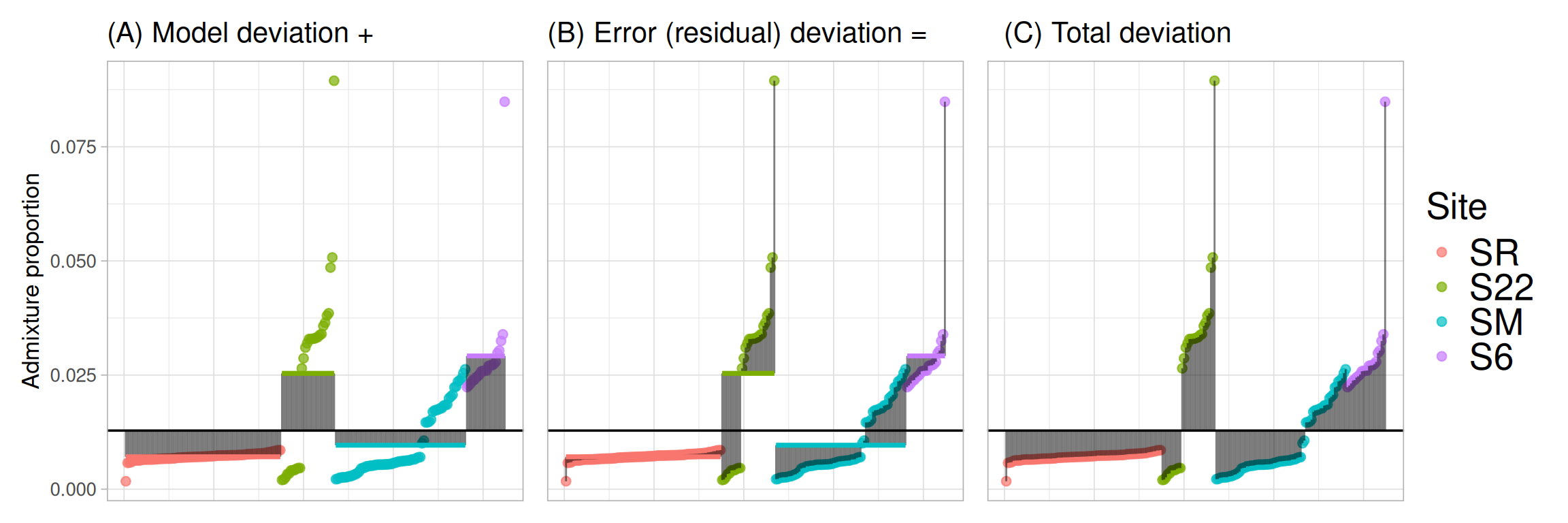

Figure 1: Partitioning the contribution of location and error to admixture proportion of plants collected from four locations. (A) Model deviation: Lines show the distance between each sample’s predicted value (i.e. group means) and the grand mean (black line). (B) Error (residual) deviation: Lines show the distance between each observation and its predicted value (i.e. group means). (C) Total deviation: Lines show the distance between each observation and the grand mean.

---

We can use the logic illustrated in Figure 1 to calculate the relevant sums of squares, and the proportion of variance explained by the model, \(r^2\):

We often see \(SS_\text{model}\) and \(SS_\text{error}\) calculated as means or variances within groups weighted by the size of each group. Those definitions are nice for rapid calculation of an ANOVA from summary statistics, but I prefer this observation-centered approach. Of course, becasue both approaches give the same answer, do what you feel.

ss_site_model <- clarkia_hz |>
  mutate(grand_mean = mean(admix_proportion))|>
  group_by(site)|>
  mutate(y_hat = mean(admix_proportion))|>
  ungroup()|>
  summarise( ss_model = sum((y_hat - grand_mean)^2),
             ss_error = sum((admix_proportion - y_hat)^2),
             ss_total = sum((admix_proportion - grand_mean)^2),
             r2       = ss_model /  ss_total,
             n        = n(),
             n_groups = n_distinct(site))

ss_model	ss_error	ss_total	r2	n	n_groups
0.0142	0.0189	0.0331	0.4298	212	4

Knowing that \(\text{DF}_\text{model} = n_\text{groups}-1\), and \(\text{DF}_\text{error} = n- n_\text{groups}\), we can find mean squares, \(F\) and our p-value:

pf() looks up our F value on the F distribution with df1 = df_model (aka df_groups), and df_2 = df_error (aka df_resid). Recall that F is a one-tailed test – we only want the upper tail (lower.tail = FALSE)

anova_results <- ss_site_model |>
  mutate(ms_model =  ss_model / (n_groups - 1),
         ms_error =  ss_error / (n - n_groups),
         F_value   =  ms_model / ms_error,
         p_value  = pf(F_value , n_groups - 1, n - n_groups, lower.tail = FALSE))

ms_model	ms_error	F_value	p_value
0.0047379	0.0000906	52.26634	3.2 x 10^-25

ANOVA in R

Of course R can do these calculations for us, with either the aov() |> summary() pipeline, or the lm() |> anova() pipeline. Both approaches yield the same result as our manual calculation, above.

aov() |> summary()

aov(admix_proportion ~ site, data = clarkia_hz)

Call:
   aov(formula = admix_proportion ~ site, data = clarkia_hz)

Terms:
                      site  Residuals
Sum of Squares  0.01421379 0.01885515
Deg. of Freedom          3        208

Residual standard error: 0.009521017
Estimated effects may be unbalanced

aov(admix_proportion ~ site, data = clarkia_hz)|>
  summary()

             Df  Sum Sq  Mean Sq F value Pr(>F)    
site          3 0.01421 0.004738   52.27 <2e-16 ***
Residuals   208 0.01886 0.000091                   
---
Signif. codes:  0 '***' 0.001 '**' 0.01 '*' 0.05 '.' 0.1 ' ' 1

lm() |> anova()

lm(admix_proportion ~ site, data = clarkia_hz)

Call:
lm(formula = admix_proportion ~ site, data = clarkia_hz)

Coefficients:
(Intercept)      siteS22       siteSM       siteS6  
   0.007094     0.018282     0.002536     0.022087  

lm(admix_proportion ~ site, data = clarkia_hz)|>
  anova()

Analysis of Variance Table

Response: admix_proportion
           Df   Sum Sq   Mean Sq F value    Pr(>F)    
site        3 0.014214 0.0047379  52.266 < 2.2e-16 ***
Residuals 208 0.018855 0.0000906                      
---
Signif. codes:  0 '***' 0.001 '**' 0.01 '*' 0.05 '.' 0.1 ' ' 1