• 15. Two-t Calculations

Motivating scenario: We want to compare means of two samples. So, we first must summarize differences in the means.

Learning goals: By the end of this section, you should be able to:

• Calculate the common summaries of two samples.
  • Means.
  • “Pooled” variance.
    
  • Cohen’s D.
    

ril_link <- "https://raw.githubusercontent.com/ybrandvain/datasets/refs/heads/master/clarkia_rils.csv"
SR_visits <- readr::read_csv(ril_link) |>
    dplyr::rename(visits = mean_visits)  |>
    dplyr::filter(location == "SR",
                  !is.na(petal_color),
                  !is.na(visits))        |>
    dplyr::select(petal_color, visits)

---

Estimates

library(ggforce)
ggplot(SR_visits, aes(x  = petal_color,
                    y    = visits,
                    fill = petal_color))+
  geom_sina(pch = 21, size = 7)+
  scale_fill_manual(values = c("pink", "white"))+
  stat_summary(fun.data   = "mean_cl_normal", linewidth = 3)+
  stat_summary(geom = "line", linewidth = 1, linetype = 2,aes(group = 1))+
  theme(legend.position = "none",
        axis.text  = element_text(size = 26),
        axis.title = element_text(size = 26))+
  labs(y = "visits")

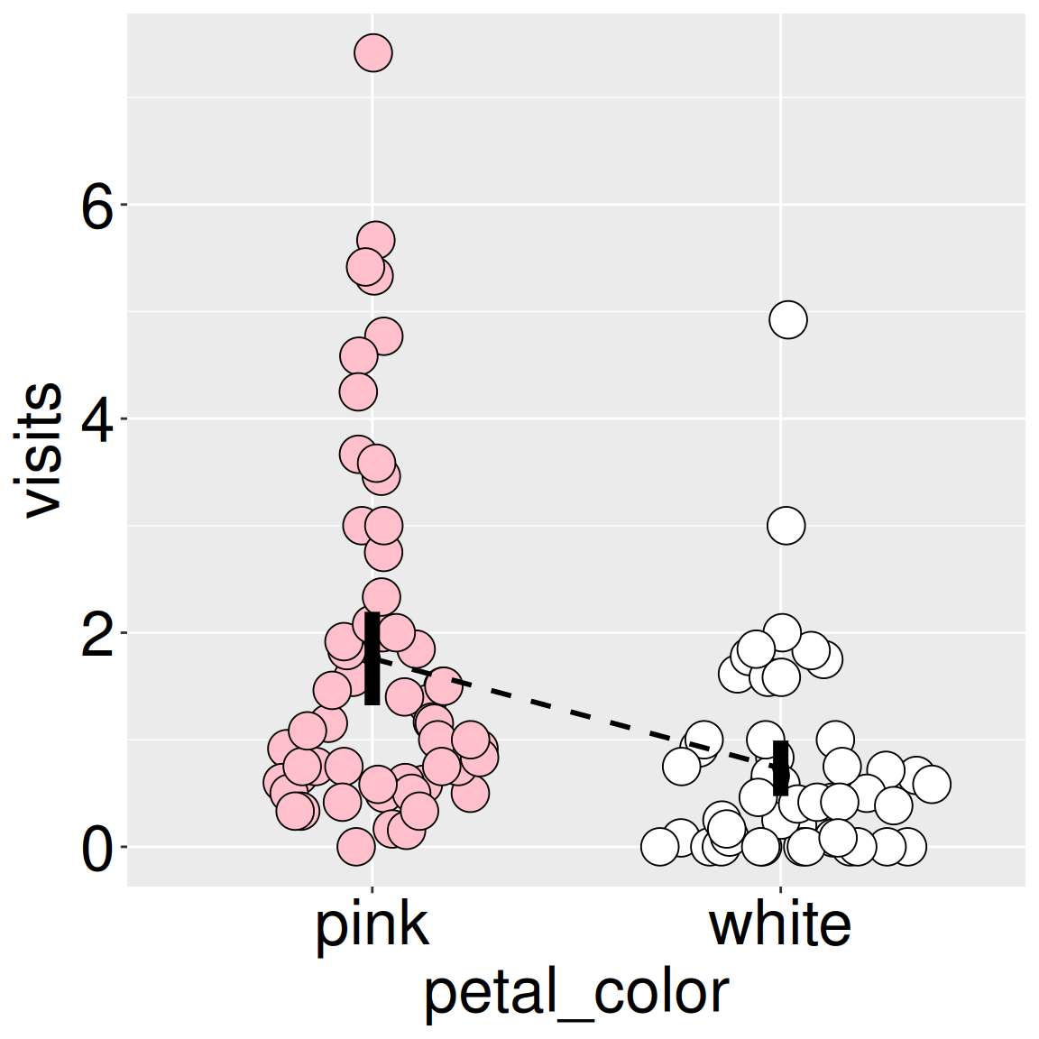
Figure 1: Each point shows an individual RIL’s mean pollinator visits. Vertical lines95% confidence intervals for each flower color. The dashed line connects the group means to facilitate comparison.

Here’s a brief refresher of our previously introduced standard summaries of associations between a categorical explanatory variable and a continuous response.

Remember that even though data do not fully meet assumptions (we can even see the right skew in the sina plot - Figure 1). Recall that if data meet assumptions of our parametric model, we can reasonably trust the results of our analysis. If data do not meet assumptions of the parametric model, results may or may not be valid, depending on how robust the test is. We will therefore conduct a permutation test and a bootstrap later to see if our t-test was trustworthy.

Estimating summaries of each group:

We can summarize within group means, and variances (or even 95% CIs, if we want) as we saw in the previous chapter. I present some of these high-level summaries in Figure 1 and calculate them below:

petal_color	MEAN	VAR	N
pink	1.759	2.710	57
white	0.733	0.833	50

color_visit_summaries <- SR_visits |>
  group_by(petal_color)|>
  summarise(MEAN  = mean(visits),
            VAR   = var(visits),
            N     = n())

Estimating summaries of differences:

We would also like to summarize the two groups jointly by estimating the pooled variance, the difference in group means, and a standardized version of that difference.

• The pooled variance: To estimate both the effect size as Cohen’s D and uncertainty, we need to calculate the variance. But we have two groups, so we need something like “the average variance within each group.” The pooled variance, \(s^2_p\) – the variance in each group weighted by their degrees of freedom and divided by the total degrees of freedom, is this average (see margin for hand calculation).

\[ \begin{align} s^2_p &= \frac{df_1 \times s^2_1 + df_2 \times s^2_2}{df_1+df_2} \\ &= \frac{(n_\text{pink}-1) \times s^2_\text{pink} + (n_\text{white}-1) \times s^2_\text{white}}{n_\text{pink}-1+n_\text{white}-1} \\ &= (56\times 2.71 + 49\times 0.833) / (56+49) \\ &= (151.76 + 40.67)/(56+49)\\ & = 192.5/105\\ &= 1.833 \end{align} \]

• The difference in means: To find this, simply subtract one mean from the other: \(\text{mean}\_\text{diff}= 1.76 - 0.733 = 1.03\).
  
  

• Cohen’s D as the difference in means standardized by the pooled standard deviation. Cohen’s D \(=\frac{\text{mean diff}}{s_p}\) \(=\frac{1.03}{\sqrt{1.833}}\) \(=\frac{1.03}{1.35}\) \(= 0.76\). This is considered a medium (borderline large) effect, so it likely matters (if true).

We can calculate these global summaries from the caculations of each petal color (above):

Size	Cohen’s D
Tiny	0.01 – 0.20
Small	0.20 – 0.50
Medium	0.50 – 0.80
Large	0.80 – 1.20
Very large	1.20 – 2.00
Huge	> 2.00

color_visit_summaries|>
    summarise(mean_diff  = diff(MEAN) |> abs(), 
              pooled_var = sum((N-1)*(VAR)) / (sum(N)-2),
              pooled_sd  = sqrt(pooled_var),
              cohens_D   = mean_diff / pooled_sd)

mean_diff	pooled_var	pooled_sd	cohens_D
1.03	1.83	1.35	0.76

The cohens_d() function in the effectsize package will calculate Cohen’s D for you! It even provides a 95% confidence interval for this estimated effect size. This package includes additional summaries of the effect size in a two-sample analysis depending on modeling assumptions. Read more here.

# Not working? Install the effectsize package!

library(effectsize) 
cohens_d(visits ~ petal_color, data = SR_visits )

Cohen's d |       95% CI
------------------------
0.76      | [0.36, 1.15]

- Estimated using pooled SD.