Motivating scenario: We fit a regression line because we want to describe how \(Y\) changes with \(X\). But we know that the line we see is only one estimate from one sample, not the true population parameter. Here, we quantify uncertainty in estimates of the slope and intercept with both mathematical and resampling-based approaches.
Learning goals: By the end of this section, you should be able to:
Explain why estimated regression slopes and intercepts vary from sample to sample.
Calculate and interpret standard errors and 95% confidence intervals for regression coefficients.
Figure 1 shows not just the data and the best fit line, but also uncertainty in this line. This follows best practices in statistical reporting – in statistics, a simple estimate of the slope or intercept is not good enough. That is because the unavoidable process of sampling error ensures that the parameters we estimate from samples will differ from true population parameters. Here we go through how to quantify this uncertainty.
Recall that we represent true population parameters with Greek letters, and estimates with English letters, so
\(a\) is our estimate of the true intercept \(\alpha\), and
\(b\) is our estimate of the true slope, \(\beta\).
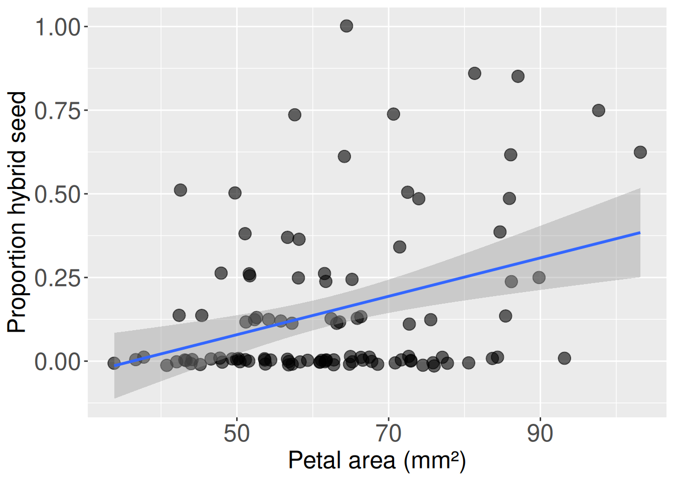
ggplot(gc_rils , aes(x = petal_area_mm, y = prop_hybrid))+geom_point() +geom_smooth(method ="lm")
Figure 1: A plot showing petal area and proportion hybrid of 103 RILs planted in GC. The blue line is the line of best fit. The shaded band around it is the 95% confidence interval for the mean of Y, prop_hybrid seeds, conditional on X, petal area.
Quantifying uncertainty from the t-distribution
Expression of critical t,\(t^*\).
For those of you who think in terms of calculus, I have added these mathematical descriptions of the critical t-value, \(t^*\). In these equations, \(f_{\text{df}}(t)\) describes the probability density of \(t\) for the specified degrees of freedom, \(df\).
We can follow standard formulas to find the standard error and 95% Confidence Intervals for the slope and intercept. So, let’s review these standard formulas:
The 95% Confidence Interval equals the parameter estimate \(\pm\) the standard error times the critical t-value. This means we need to find both the critical t value and the standard error to calculate the 95% confidence interval
The critical t-value, \(t^*\), tells us how many standard errors we need to move away from the center to capture the middle \(1-\alpha\) of a \(t\)-distribution with a given number of degrees of freedom. The area between the negative and positive critical values is \(1-\alpha\), while the remaining area, \(\alpha\), is split equally between the two tails of area \(\frac{\alpha}{2}\).
The degrees of freedom error equals the sample size minus the number of parameters estimated in the model. Because a linear regression estimates two parameters (the slope and intercept), a linear regression has \(n-2\) degrees of freedom error.
So now we just need formulas for the standard errors of the slope and intercept and we can find the 95% confidence intervals!
Uncertainty in the slope
The standard error of the slope, \(SE_b\), is one divided by the square root of \((n-2)\), times the ratio of standard deviation in residuals, \(s_e\), to standard deviation in X, \(s_X\). We can now find the SE and 95% CI of the slope on our own in R:
The standard error in the intercept, \(SE_a\), is not easy to wrap our heads around intuitively. So I simply present this equation on the right, and hold on tight as we turn the crank in R:
We can avoid these calculations altogether! R will return the standard errors with the summary() function and the confidence intervals with the confint() function. Or, more concisely, R will return both with broom’s tidy() function:
To avoid distracting you, I did not show you the p-value (select(-p.value)). We will learn how to find p-values, test null hypotheses, and interpret these results in the next section.
Call:
lm(formula = prop_hybrid ~ petal_area_mm, data = gc_rils)

Residuals:
     Min       1Q   Median       3Q      Max
-0.32681 -0.14608 -0.05947  0.08676  0.83802

Coefficients:
               Estimate Std. Error t value Pr(>|t|)
(Intercept)   -0.207834   0.099466  -2.089 0.039176 *
petal_area_mm  0.005738   0.001555   3.691 0.000362 ***
---
Signif. codes:  0 '***' 0.001 '**' 0.01 '*' 0.05 '.' 0.1 ' ' 1

Residual standard error: 0.2246 on 101 degrees of freedom
Multiple R-squared:  0.1188,    Adjusted R-squared:  0.1101
F-statistic: 13.62 on 1 and 101 DF,  p-value: 0.0003625
Bootstrap-based uncertainty
Because our data do not fit assumptions of the linear model particularly well (see previous section), we must find a way to see how much we can trust the estimates of uncertainty calculated above. Bootstrapping – that is, resampling our data with replacement, estimating the slope and intercept of this “bootstrapped” dataset, and repeating this many times, provides an alternative way to estimate uncertainty without relying on the assumptions of the t-distribution.
These bootstrap-based estimates are quite close to our t-based summaries (Intercept: SE = 0.0995, 95% CI = {-0.4051 , -0.0105}, Slope: SE = 0.0016, 95% CI = {0.0027 , 0.0088}).
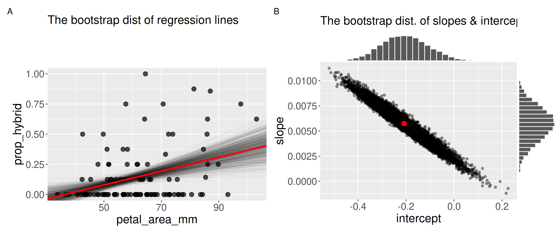
Figure 2 also reveals something interesting – our estimates of the slope and intercept are non-independent. When we overestimate the slope we will tend to underestimate the intercept and vice-versa. This makes sense when you think for a minute, but is not obvious in our linear summaries above.
Figure 2: Bootstrapped uncertainty in a linear regression. Panel A shows the observed relationship between petal area and proportion hybrid seed, with the fitted regression line in red and 1,000 bootstrapped regression lines in gray. Panel B shows the bootstrap distribution of the estimated intercepts and slopes from many resampled datasets. The red point marks the slope and intercept from the original dataset.
Optional
Uncertainty in predictions
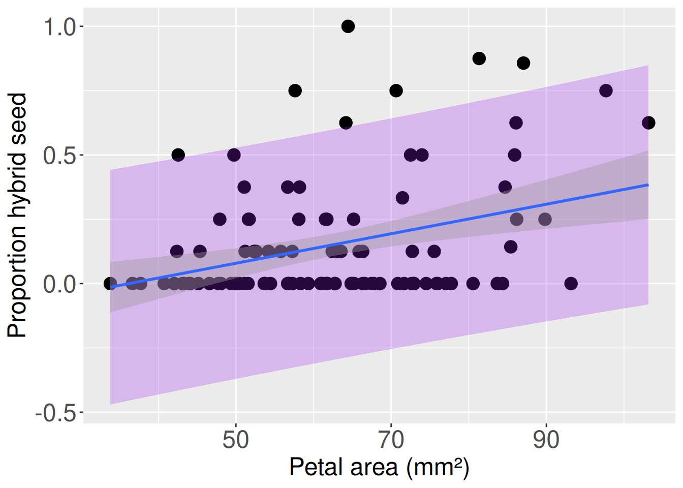
We often think of a regression line as “predicting” the value of the response variable, given the value of the explanatory variable. But what exactly is being predicted? The fitted value, \(\widehat{Y_i}\), is our estimate of the mean value of \(Y\) for observations with a given value of \(X\). In this example, the regression line estimates the mean proportion hybrid for RILs with a given petal area (Figure 1). The confidence interval around the regression line shows uncertainty in this estimated mean. But this is not the same as predicting where a new individual observation will fall.
If we want a range where we expect a new observation of \(Y\) to fall, conditional on \(X\), we use a prediction interval. As seen in Figure 3, prediction intervals are wider than confidence intervals because they describe uncertainty for individual observations. This figure also highlights problems with this model: all points that fall outside the prediction interval are above it, and much of the prediction interval extends below zero. I dont need a standard error to know that’s wrong. We will address these issues with more flexible models in a later chapter.