Enjoy this “insomnia meme” about the ANOVA. From this video
We previously introduced F and the ANOVA approach as an alternative to the two sample t-test. Here we show its true utility - by testing the single null hypothesis that all samples come from the same statistical population, we avoid the “multiple testing problem.” As such, compared to the naive testing of all pairwise differences, the ANOVA approach allows us to fairly test for differences in means among numerous groups. If we reject the null that all groups are equal, we conduct a “post-hoc” test to see which groups differ.
Chatbot tutor
Please interact with this custom chatbot (ChatGPT link here,Gemini link here). I have made it to help you with this chapter. I suggest interacting with at least ten back-and-forths to ramp up and then stopping when you feel like you got what you needed from it.
Practice Questions
Try these questions! By using the R environment you can work without leaving this “book”. I even pre-loaded all the packages you need!
Setup
Fiddler males have a greatly enlarged “major” claw, which is used to attract females and to defend a burrow. Darnell and Munguia (2011) suggested that this appendage might also act as a heat sink, keeping males cooler while out of the burrow on hot days. To test this, they placed four groups of crabs into separate plastic cups and supplied a source of radiant heat (60-watt light bulb) from above. The four groups were intact male crabs; male crabs with the major claw removed; male crabs with the other (minor) claw removed (control), and intact female fiddler crabs. They measured body temperature of crabs every 10 minutes for 1.5 hours. These measurements were used to calculate a rate of heat gain for every individual crab in degrees C/log minute.
Rates of heat gain for all crabs are loaded here as crabs but can be downloaded from this link: https://raw.githubusercontent.com/ybrandvain/datasets/refs/heads/master/crabs.csv
Q1.a) There are four groups. How many potential pairwise comparisons are there? .
For 4 groups, the number of unique pairs is: \[\frac{k(k - 1)}{2} = \frac{4(3)}{2} = 6\]
Q1.b) Assume all samples come from the same population (i.e. the null hypothesis is true). If we conducted all pairwise tests and rejected a null if the p-value was less than 0.05, what is the probability of rejecting at least one true null across all of these pairwise tests?
The probability of not incorrectly rejecting a true null is 0.95. To not falsely reject any true nulls we need six such successes. \[0.95^6 \approx 0.735\] So the probability of incorrectly rejecting at least one true null is:
\[1 - 0.735 = 0.265 \]
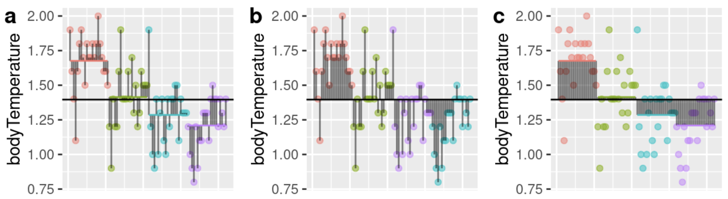
Q2) Consider the plot above. Before running an ANOVA or post-hoc test, which comparison do you think is most likely to be significantly different?
Calculate the sample size, mean, and variance for each treatment
Q3) Compare the variance within each treatment. What is the greatest fold difference in variance between treatments?
Q4) With this difference in variance among groups, the assumption of homoscedasticity is
Figure 1: Three panels (a–c) show body temperature measurements for individual crabs across four treatment groups. Points represent individual observations, horizontal colored segments indicate group means, and vertical black lines show deviations between observations and means or between means and the overall mean.
Q5) Consult Figure 1 to answer the questions below:
Q5.a) Which panel in Figure 1 shows total deviations? . Q5.b) Which panel in Figure 1 shows model deviations? . Q5.c) Which panel in Figure 1 shows error deviations? .
Assume we were using the code below to build an ANOVA for the crabs data
Q6) What would be the best name for this_partition?
Q7.a) Why didn’t the code above work?
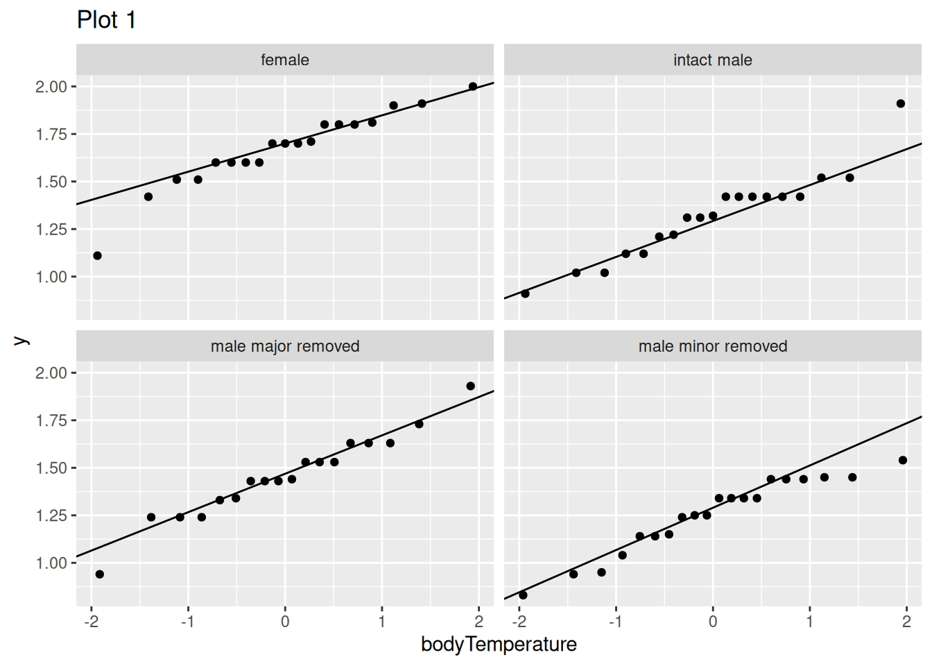
Plot 1: Normal Q–Q plots of body temperature values for each crab group, shown separately by crab type.
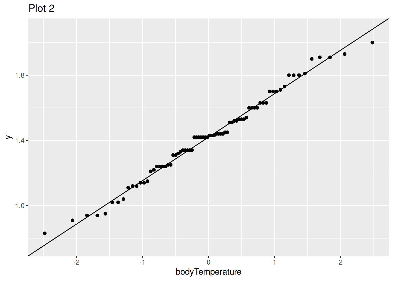
Plot 2: Normal Q–Q plot of all body temperature values pooled across crab types.
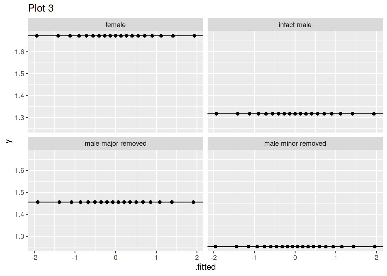
Plot 3: Normal Q–Q plots of model-predicted values for each crab group.
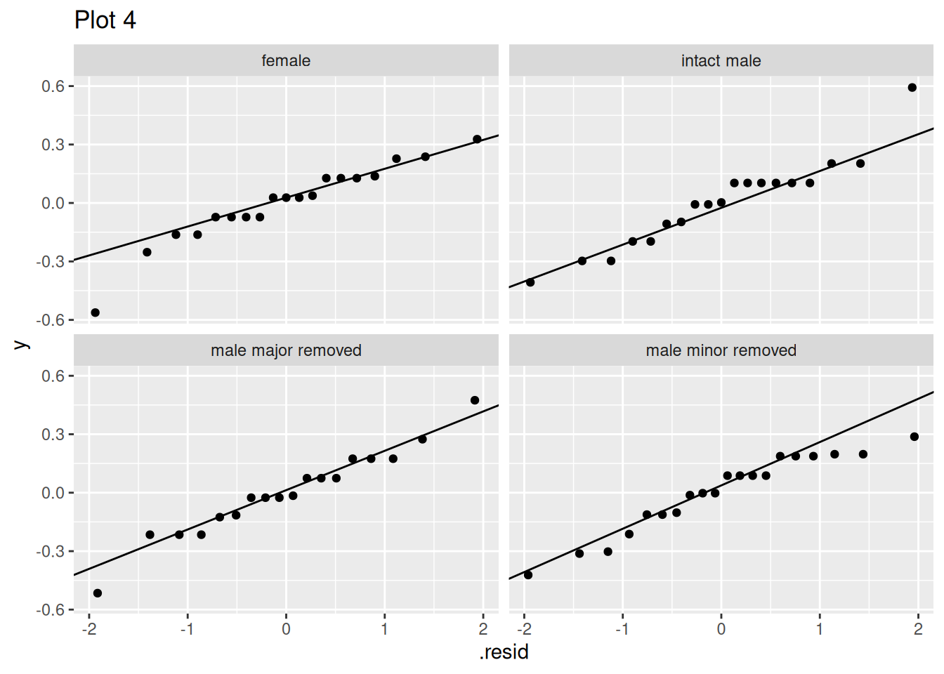
Plot 4: Normal Q–Q plots of deviations between observed and predicted values for each crab group.
Q7.b) Fixing this error, which assumption are these plots meant to evaluate?
Q7.c) Which two of the plots are reasonable ways to evaluate this assumption.
Q8) In the context of an ANOVA, which R code gives you:
Q8.a) Estimates of model coefficients ONLY?
Q8.b) An ANOVA table
Q8.c) Results of a post-hoc test (Note there are other post-hoc options too)
Q8.d) Model coefficients and standard errors, plus numerous potentially misleading p-values and t-values that should largely be ignored
Run the relevant statistical tests below
Q9) Run an ANOVA on the data. What do we do to the null hypothesis?
Q10) According to the post-hoc test, if female is in significance group, “a”, which group(s) is intact male major in?
Let’s work through this one, because it wasn’t easy.
First we run our model, and conduct our post-hoc test:
# Load Datacrab_link <-"https://raw.githubusercontent.com/ybrandvain/datasets/refs/heads/master/crabs.csv"crabs <-read_csv(crab_link)# Format datacrabs <-mutate(crabs , crabType=factor(crabType))# Analyze dataaov(bodyTemperature ~ crabType, data = crabs)|>TukeyHSD()
                             comparison     p.adj
1                    intact male-female 0.0000134
2             male major removed-female 0.0144778
3             male minor removed-female 0.0000002
4        male major removed-intact male 0.2083508
5        male minor removed-intact male 0.7778607
6 male minor removed-male major removed 0.0228208
Let’s hone in on the comparisons with p.adj\(< 0.05\) (i.e., where we reject the null hypothesis).
We see that female significantly differs from everyone else (all comparisons involving female have p.adj\(< 0.05\)). So we put female in significance group a. Because female differs from all other groups, no other groups are in significance group a.
The post-hoc test reveals one more significant difference — male minor removed differs from male major removed. So, we place one in group say b and one in group c (it doesn’t matter which is which).
Finally, intact male only differs significantly from female. So, it cannot be in group a, but it does not differ from either male minor removed or male major removed. So, intact male belongs to both significance groups b and c.
📊 Glossary of Terms
Multiple Testing Problem: The inflation of the false positive rate when conducting many hypothesis tests simultaneously.
One-way ANOVA: A comparison of means across more than two groups.
Residual: The difference between an observation and its value predicted by the linear model.
Homoscedasticity: Equal variance across groups.
Between-Group Variation (\(\text{SS}_\text{model}\)): Variation explained by differences among group means. \(\text{SS}_\text{model} = \Sigma{(\hat{Y_i} - \bar{Y})^2}\). We can also find \(\text{MS}_\text{model}\) by dividing \(\text{SS}_\text{model}\) by \(df_\text{model}\), where \(df_\text{model}\) is the number of terms in our linear model.
Within-Group Variation (\(\text{SS}_\text{error}\)): Variation among observations within each group. \(\text{SS}_\text{error} = \Sigma{(Y_i-\hat{Y_i})^2}\). We can also find \(\text{MS}_\text{error}\) by dividing \(\text{SS}_\text{error}\) by \(df_\text{error}\), where \(df_\text{error}\) is the number of observations minus the number of terms in our linear model.
F Statistic: Ratio of between-group to within-group variance: \(F = \frac{\text{MS}_\text{model}}{\text{MS}_\text{error}}\).
\(R^2\): Proportion of total variance explained by the model. \(R^2 = \frac{SS_\text{model}}{SS_\text{total}}\).
Post-hoc Test: A follow-up test conducted after rejecting ANOVA’s null hypothesis to determine which specific groups differ.
Significance Groups: A compact way to summarize post-hoc results using letters; groups sharing a letter are not significantly different.
📦 R Packages Introduced
[broom](broom: A collections of functions to tidy the outputs of a linear model, including; tidy(), augment(), and glance().
multcomp. A packge with numerous tools for multiple comparisons, including general linear hypothesis testing (glht()) and functions to generate significance groupings (cld()).
rstatix A package for statistical tests, including post-hoc procedures like the Games–Howell test (games_howell_test()).
Hmisc: An R package with “miscellaneous” functions. In this chapter, it is used formean_cl_normal, which works with stat_summary() to add means and confidence intervals to plots.
🛠️ Key R Functions
lm(): Fits a linear model, which is the underlying framework for ANOVA. Running lm(y ~ group), fits an ANOVA, where group means are expressed through coefficients.
anova(): Produces an ANOVA table from a fitted model (typically from lm()). It partitions variation into components (model vs. error) and reports sums of squares, mean squares, the F statistic, and p-values.
summary(). Summarizes a fitted lm() model, providing coefficients, standard errors, t-values, and p-values. In ANOVA contexts, these p-values are often misleading for multi-group comparisons and should be ignored.
aov(): Like lm(), aov Fits an ANOVA model using a formula (e.g., y ~ group). Unlike lm the output is designed to work with one way ANOVA-style analyses and to integrate with functions like TukeyHSD() for post-hoc testing, but does not provide coefficients for a linear model.
TukeyHSD(): Performs Tukey’s post-hoc test following an ANOVA fit with aov().
glht(): Conducts general linear hypothesis tests, including Tukey-style post-hoc comparisons, from models fit with lm(). It is more flexible than TukeyHSD() and works with a wider range of models.
oneway.test(): Conducts Welch’s ANOVA, which does not assume equal variance across groups. Use games_howell_test() for the corresponding post-hoc test.
games_howell_test(): Performs a post-hoc test that does not assume equal variance among groups. It is typically used after Welch’s ANOVA (i.e. output from oneway.test()) and is robust to heteroscedasticity.
cld(): Converts post-hoc test results (e.g., from glht()) into significance groups (a, b, etc.) that summarize which groups differ.
augment(): Adds model outputs (e.g., fitted values and residuals) back onto the original dataset.
tidy():Converts model output into a clean, tabular format.
Chapters 16, 17 and 18 of “Introduction to Statistics and Data Analysis” by Geoffrey M. Boynton.
Comparing several means (one-way ANOVA) from Learning statistics with R: A tutorial for psychology students and other beginners. (Version 0.6.1) Danielle Navarro.