library(car)
library(ggplot2)
library(dplyr)
library(honestlm)
library(emmeans)
library(modelbased)
library(parameters)
library(broom)
penguins <- penguins |>
filter(!is.na(sex),!is.na(body_mass),!is.na(flipper_len))• 20. Multiple Regression in R
.
Motivating example: Throughout this section I have sprinkled in R code about how to do things, but this code was mixed with explanations, theory, and the like. Now that you understand the concepts of a multiple regression, you want a quick resource about how to do this in R.
Learning goals: By the end of this section, you should be able to:
- Complete a first-pass analysis of data.
This is not enough
Just copying and pasting code from this section will not be a strong analysis. Please read the entire chapter! Rather, this serves as a “first-pass” resource for a more detailed analysis.
Getting started with multiple regression
Let’s first load the key packages we use to assist us in multiple regression:
Model building
For this example, I will take the penguins data set and model flipper length as a function of body mass, sex, and species.
full_model <- lm(flipper_len ~ body_mass  + species +  sex, data = penguins)
coef(full_model)| (Intercept) | body_mass | speciesChinstrap | speciesGentoo | sexmale |
|---|---|---|---|---|
| 165 | 0.00655 | 5.54 | 18 | 2.48 |
From these coefficients, we can build a linear model.
\[ \widehat{\text{flip len}_i} = 165 + 0.00655 (\text{body mass}_i) + 5.54 (\text{Chinstrap}_i) + 18 (\text{Gentoo}_i) + 2.48 (\text{male}_i) \]
Remember that levels of categorical “indicator variables” (e.g. male, Gentoo, etc) are 0 if you are not that thing, and 1 if you are. So, for example, an Adelie female has a flipper length of \(165+0.00655 \times \text{its body mass}\), while an Adelie male has a flipper length of \(165 + 2.48+0.00655 \times \text{its body mass.}\)
Visualization
The next step is to look at the data. Remember that
- There are numerous ways to visualize multivariate data.
- Slopes and means from
geom_smooth()andstat_summary(), respectively, are specific to each group and do not necessarily correspond to predictions from a simple additive model.
So, rather than making you a static plot, I am providing this webR environment, with my honestlm package loaded, with geom_lm_smooth() and stat_lm_means() ready to go!
Have a look at the output and see what you notice. Then try swapping mapping of sex and species (i.e. facet by sex and color by species). Then try putting body mass on the y. What do you notice? How does this guide your understanding of the data and model?
Evaluating assumptions
Now we are ready to evaluate assumptions.
- First we can evaluate the possibility of multicollinearity with the
vif()function from thecarpackage:
vif(full_model) GVIF Df GVIF^(1/(2*Df))
body_mass 6.527137 1 2.554826
species 5.349026 2 1.520788
sex 2.124967 1 1.457727While we see some association among predictors, these are just on the edge at which we start to take notice. I don’t think we’re fully in the danger zone yet.
- Next we evaluate assumptions of linearity, normality of residuals, and homoscedasticity with diagnostic plots:
plot(full_model)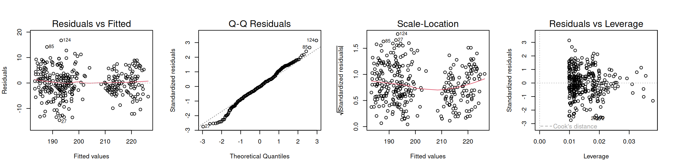
These plots all seem reasonably good. There is a slight deviation from normality assumptions but this does not worry me!
Parsing effect sizes
We can now compare effect sizes with the partial_r2() function in my honestlm package.
partial_r2(full_model)# A tibble: 3 × 4
term df partial_r2 f2
<chr> <dbl> <dbl> <dbl>
1 body_mass 1 0.131 0.151
2 species 2 0.351 0.542
3 sex 1 0.0250 0.0257We see that compared to species and body mass, sex explains a relatively small proportion of individual variation in flipper length, after adjusting for all associations among explanatory variables.
Evaluating significance
Making sure to use car’s Anova() function, we find strongly significant association between all explanatory variables and flipper length, even after adjusting for associations among explanatory variables.
Anova(full_model, type = "II")Anova Table (Type II tests)
Response: flipper_len
Sum Sq Df F value Pr(>F)
body_mass 1414.9 1 49.5157 1.155e-11 ***
species 5075.7 2 88.8174 < 2.2e-16 ***
sex 240.5 1 8.4165 0.00397 **
Residuals 9372.3 328
---
Signif. codes: 0 '***' 0.001 '**' 0.01 '*' 0.05 '.' 0.1 ' ' 1With a post-hoc test, we find that the flipper length of all species differ from one another after adjusting for associations between explanatory variables.
emmeans(full_model, ~ species) |>
  contrast(method = "pairwise", adjust = "tukey")
contrast estimate SE df t.ratio p.value
Adelie - Chinstrap -5.54 0.785 328 -7.061 <0.0001
Adelie - Gentoo -18.02 1.440 328 -12.493 <0.0001
Chinstrap - Gentoo -12.48 1.500 328 -8.333 <0.0001
Results are averaged over the levels of: sex
P value adjustment: tukey method for comparing a family of 3 estimates Summarizing uncertainty
Here, I will only use the model_based and the related parameters (both in the easystats family of packages) packages to summarize uncertainty. This deviation from the text just shows you other ways to do things! Pick your favorite.
- Uncertainty in model coefficients:
model_parameters(full_model)| Parameter | Coefficient | SE | 95% CI | \(t_{328}\) | \(p\) |
|---|---|---|---|---|---|
| (Intercept) | 165 | 3.18 | [158, 171] | 51.7 | <0.001 |
| body_mass | 0.00655 | 0.000931 | [0.00472, 0.00838] | 7.04 | <0.001 |
| speciesChinstrap | 5.54 | 0.785 | [4.00, 7.09] | 7.06 | <0.001 |
| speciesGentoo | 18.0 | 1.44 | [15.2, 20.9] | 12.5 | <0.001 |
| sexmale | 2.48 | 0.854 | [0.798, 4.16] | 2.90 | 0.004 |
Ignore these p-values
Remember, the p-values here refer to the deviation of model coefficients from a null value of zero. This is rarely what we care about. I suggest ignoring them. For term-level tests, use the Type II sums of squares approach above.
- Uncertainty in adjusted means:
estimate_means(full_model, by="sex")| sex | Mean | SE | 95% CI | t | df |
|---|---|---|---|---|---|
| female | 200 | 0.547 | [199, 201] | 366 | 328 |
| male | 202 | 0.508 | [201, 203] | 399 | 328 |
estimate_means(full_model, by="species")| species | Mean | SE | 95% CI | t | df |
|---|---|---|---|---|---|
| Adelie | 193 | 0.643 | [192, 195] | 301 | 328 |
| Chinstrap | 199 | 0.784 | [197, 200] | 254 | 328 |
| Gentoo | 211 | 0.952 | [210, 213] | 222 | 328 |