• 17. Multiple testing problem
Motivating Scenario: Your sample has data from more than two groups, and you want to know if group means differ from one another. This section explains why you cannot simply conduct all possible pairwise t-tests, and why you should instead use an ANOVA framework.
Learning Goals: By the end of this subchapter, you should be able to:
Explain how conducting multiple tests inflates the overall (experiment-wise) false positive rate.
Describe how ANOVA addresses the multiple testing problem by reframing it as a single hypothesis test.
Know that there are alternative approaches to solve the multiple testing problem.
Multiple tests make a liar of your p-value
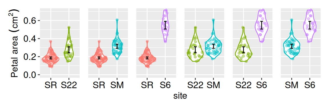
There are \({4 \choose 2} = 6\) possible pairwise comparisons of mean petal areas among the four Clarkia xantiana parviflora hybrid zone populations we studied (Figure 1). Even when all six nulls are true, there’s roughly a one in four chance that at least one test will falsely appear ‘significant.’ That’s because the probability all six avoid a false positive is \(0.95^6 = 0.735\).
Thus for this study, the probability of at least one false positive is \(1 - 0.735 = 0.265\), a value much larger than the \(\alpha = 0.05\) that was advertised. This problem gets pretty bad pretty quick (Figure 2). As such, conducting many t-tests on the same data makes your p-values misleading—they no longer represent the 5% false-positive rate we usually assume. When you run multiple tests, the chance of seeing at least one ‘significant’ result just by luck is much higher, so the reported p-values give a false sense of confidence
the probability of at least one false positive is 0.265
More broadly, the number of pairwise comparisons between n groups equals
\(n_\text{pairs} = \binom{n}{2} = \frac{n (n-1)}{2}\), and the experiment-wise false positive rate equals, \(1-(1-\alpha)^{n_\text{pairs}}\).
comparisons <- tibble(n_groups= 2:15)|>
    mutate(n_comparisons = choose(n_groups,2),
           experiment_alpha = 1-.95^n_comparisons)

ggplot(comparisons, aes(x = n_groups,  y =experiment_alpha))+
    geom_point(size= 4)+
    geom_line(linetype = 3, linewidth = 1.4)+
    labs(x = "# groups",
         y = "P(≥ 1 false positive)",
         title ="The multiple testing problem")+
    theme(axis.text = element_text(size = 23),
          title = element_text(size = 23),
          axis.title = element_text(size = 23))+
    scale_x_continuous(breaks = seq(2,14,2))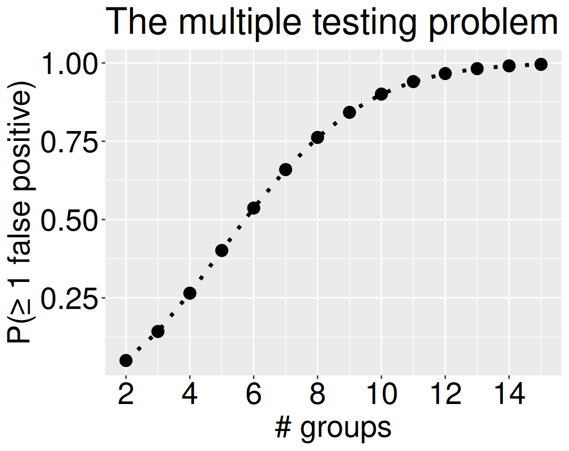
ANOVA avoids the multiple testing problem
For p-values to be worth anything, they should correspond to the problem we set up. There are numerous ways to address the multiple testing problem (see below, and Wikipedia).
Instead of testing each combination of groups separately, ANOVA poses and tests a single null hypothesis — that all samples come from the same statistical population. This results in a well-calibrated null model (i.e. we will reject a true null with probability \(\alpha\)).
ANOVA hypotheses
- \(H_0\): All samples come from the same (statistical) population. Practically, this means that all groups have the same mean.
- \(H_A\): Not all samples come from the same (statistical) population. Practically this says that not all groups have the same mean.
But how do we see which groups differ? Our scientific hypotheses and interpretations depend not just on the single null hypothesis – “all groups are equal”– but on knowing which groups differ from one another. Later in this chapter we will introduce “post-hoc tests”, which ask “which groups differ from one another?” Importantly, post-hoc tests should only be used after we reject the null that all groups have the same mean.
Other ways to handle multiple comparisons
ANOVA solves the multiple-testing problem by asking one big question instead of many small ones. However, sometimes we really do need to test many hypotheses. For example, when comparing every pair of groups, analyzing many traits, or in genome-wide association studies etc. we are testing multiple hypotheses. So there are other approaches to deal with this issue.
The Bonferroni correction is the simplest correction for multiple tests. A Bonferroni correction creates a new \(\alpha\) threshold by dividing your stated \(\alpha\) by the number of tests. So, if you test five different nulls at an \(\alpha = 0.05\), the Bonferroni correction will reject a null when \(p<\frac{0.05}{5}=0.01\).
As the number of comparisons increases this correction becomes overly conservative, so people turn to other methods.
The False Discovery Rate (FDR) Rather than considering any false positive, FDR-based corrections consider the expected proportion of false positives among the results we call significant. So, an FDR-based correction ensures that, on average, about 5% of the results we call ‘significant’ are actually false positives.