• 10. Statistical Hypotheses

Motivating Scenario: You are beginning your journey into the world of null hypothesis significance testing. Wait… what even is a null hypothesis?

Learning Goals: By the end of this section, you should be able to:

Explain why we create null models and what makes a good one.
Differentiate between the null and alternative hypothesis.
Differentiate between biological and statistical hypotheses.

A comic shows two stick figures talking. One says, *I cant believe schools are still teaching kids about the null hypothesis.* The second figure responds, *I remember reading a big study that conclusively disproved it years ago.* In the background, a child sits at a desk, appearing to work on something. — Figure 1: From xkcd. *Rollover text:* Heck, my eighth grade science class managed to conclusively reject it just based on a classroom experiment. Its pretty sad to hear about million-dollar research teams who can’t even manage that.

Scientific hypotheses are exciting. As scientists, we ask interesting questions. For example, throughout this book, we are asking if parviflora flowers have evolved in ways to make them less likely to make hybrids with their close relative, xantiana. Other scientific questions include: Do vaccines cause autism? Does a novel drug have its claimed effect? These are examples of scientific hypotheses. These are our scientific hypotheses. They are meaningful, and grounded in our understanding of the biological world. They are the reason we do science.

As scientists, we’re usually trying to evaluate support for a scientific hypothesis. But in the null hypothesis significance testing framework of frequentist statistics (which we follow for most of this book), we do this in a somewhat backwards way. We evaluate the plausibility of a boring statistical hypothesis, known as the null hypothesis. If our observations are inconsistent with the null, we conclude that there is likely something else going on.

The null hypothesis

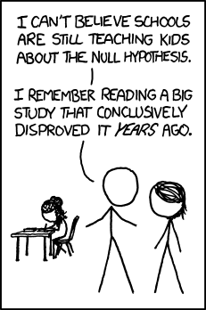
The Null Hypothesis (\(H_0\)) is the ultimate skeptic. It argues that any pattern you see in your data is just an illusion created by random chance or sampling error. It’s the voice that says, “nothing interesting is happening here” (Figure 2). This is a very specific claim so the null model is very specific.

Russell Westbrook dramatically yawning, with the text 'Cool story, bro.' at the bottom. — Figure 2: The null hypothesis is unimpressed by your sampling error.

The Alternative Hypothesis (\(H_A\) or \(H_1\)) is the claim that the null hypothesis is not true. It claims that something other than random sampling error is responsible for the observed pattern. This is a vague claim. So the alternative hypothesis is not making a specific claim – its just there as a grab bag for all not in the null..

The Alternative Hypothesis (\(H_A\) or \(H_1\)) is the claim that the null hypothesis is not true — that something other than random sampling error is responsible for the observed pattern.

For our flower example, the null and alternative hypotheses are:

\(H_0\): The proportion of moms with at least one hybrid seed does not differ between white and pink flowered plants.
\(H_A\): The proportion of moms with at least one hybrid seed does differ between white and pink flowered plants.

The null hypothesis doesn’t care about your theories, it does not evaluate effect size, and has no sense of biological relevance.

Properties of good null hypotheses

Notice that we chose to compare proportions, not the raw counts of plants with hybrids. This is a crucial feature of a good hypothesis test: it must make a fair comparison. Because our sample sizes for pink (56) and white (58) flowers were unequal, comparing raw counts would be misleading and biologically uninteresting. More generally, because the null hypothesis is a skeptic that doesn’t understand biology, it’s our job to design studies where its rejection is both interesting and informative.

Good nulls are non-trivial: Testing the null that white flowers have zero hybrids is lame. If we see at least one hybrid then we couldn’t have gotten such a result by sampling error from a population with no hybrids. Similarly, the null hypothesis that mean petal length is zero mm squared should not be tested!
Good nulls represent a fair comparison: As stated above, we compared the proportion of white and pink flowered plants with at least one hybrid seed, not the raw counts to avoid bias. When you design your studies make sure the comparison is fair!
Great nulls isolate the effect of interest: A great null model creates a world where “all else is equal” (ceteris paribus). For example, the best test would ensure that other covariates, that differ (e.g. differences in petal length) between our explanatory variable (e.g. flower color morph), aren’t the real cause of a difference in our response variable.

tl/dr: Take-home message: It is our responsibility to design studies that create a clear link between our exciting scientific questions and the rigid framework of statistical testing.

Check out this fun PhD Comic on the "Analysis of Value" on the analysis of value for a related laugh.

One tail, two tails, red tail blue tail.

Two panels comparing rejection regions for hypothesis tests using a normal null distribution centered at zero. In the left panel, representing a two-tailed test, dashed vertical lines mark symmetric critical values on both sides of the distribution. The shaded regions beyond these lines represent the rejection regions, each labeled α/2. In the right panel, representing a one-tailed test, a single dashed vertical line marks the critical value on the right side of the distribution, and the shaded region beyond it represents the rejection region labeled α. Both panels label the horizontal axis as the test statistic under the null hypothesis. — Figure 3: **One- vs. two tailed test of the null hypothesis.** Both panels show a null distribution for a test statistic centered at zero. In the two-tailed test (left), the significance level α is split evenly between both tails of the distribution, so each tail contains α/2 of the probability. In the one-tailed test (right), the entire significance level α lies in a single tail of the distribution. We reject the null hypothesis when the observed test statistic falls in the shaded tail.

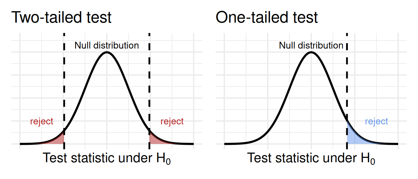
Figure 1 shows the difference between a one- and two- tailed test. We almost always use a two-tailed test – in which we note deviations from the null in either direction, unless one of the directions is completely meaningless. For example:

Above, we conducted a two-tailed test of the null hypothesis. According to this, standard practice, thee null is that proportions “differ” between white and pink morphs. It did not specify a direction. In a wo tailed test, we are open to the effect going in either direction.
A one-tailed test is when we only care about a specific direction (e.g., \(H_A\): pink flowers have a higher proportion of hybrids). In practice, one-tailed tests are rare and often inappropriate because we’d almost always want to know about a strong effect in the unexpected direction. Additionally, one-tailed tests often breed distrust in your audience – they signal that you are trying to pull a fast one.

Rare cases when a one-tailed test is appropriate occur when both extremes of the outcome are on the same side of the null distribution. For instance, if I were studying the absolute value of something, the null hypothesis would be that it’s zero, and the alternative would be that it’s greater than zero. We’ll see that some test statistics, like the \(F\) statistic and (often) the \(\chi^2\) statistic, only have one relevant tail.