• 12. Two predictors

Motivating Scenario:
You noticed that two variables (e.g. petal color and petal area) are associated with the response variable (e.g. the proportion of hybrid seeds). You want to know how to build one model that includes both.

Learning Goals: By the end of this section, you should be able to:

Fit a general linear model with two predictors
- Build a model with both continuous and categorical explanatory variables with R.
Interpret coefficients in a two-predictor model
- Understand the meaning of intercepts, slopes, and group differences.
Manually calculate predicted values and residuals
- Predict responses for individuals and compute residuals from model output.

Code for selecting data from a few columns from RILs planted at GC

ril_link <- "https://raw.githubusercontent.com/ybrandvain/datasets/refs/heads/master/clarkia_rils.csv"
ril_data <- readr::read_csv(ril_link) |>
  dplyr::mutate(growth_rate = case_when(growth_rate =="1.8O" ~ "1.80",
                                          .default = growth_rate),  
                growth_rate = as.numeric(growth_rate),
                visited = mean_visits > 0)
gc_rils <- ril_data |>
  filter(location == "GC", !is.na(prop_hybrid), ! is.na(mean_visits))|>
  select(petal_color, petal_area_mm, num_hybrid, offspring_genotyped, prop_hybrid, mean_visits , asd_mm,visited )|>
  mutate(log10_petal_area_mm = log10(petal_area_mm))

We found that both petal area and petal color predict the proportion of hybrid seeds in parviflora RILs. We’ve seen how to model each relationship individually, but what if you want to consider both traits at once? Does petal size still matter when accounting for petal color? Or does petal color ‘explain away’ the apparent association of proportion hybrid seeds with petal size?

The “general linear model” allows us to tackle such questions by modeling multiple explanatory variables at once. To do so, we extend our familiar simple linear model to include both kinds of predictors at once.

Mathematically, the prediction for an individual becomes:

\[\hat{y}_i = b_0 + b_1 x_{1i} + b_2 x_{2i}\] Let’s work through this as applied to our case:

$y$ as proportion of hybrid seed.
$b_0$ is the intercept… i.e. the proportion of hybrid seeds for a pink-petaled plant with petal area equal to zero.

$b_0$ is biological nonsense, of course. A flower with a petal area of zero wouldn’t have a color, let alone attract pollinators. The intercept here is a statistical and mathematical construct — not a biological claim. That’s ok! Just make sure to never use a linear model to make predictions beyond the range of your data.

$x_{1i}$ as petal area of RIL $i$.
$b_1$ is the slope — the expected change in the proportion of hybrid seeds, for every unit increase in petal area (as in the previous chapter). Note that this assumes that pink and white flowers have the same slope. We revisit this later.
$x_2$ as the indicator variable for petal color, which equals 0 for pink petaled-flowers and 1 for white-petaled flowers (i.e. pink is the “reference level”).
$b_2$ is the difference in the intercepts for white- and pink- petaled flowers i.e. the difference in the expected proportion of hybrid seeds for pink and white petaled-flowers with the same petal area.

With this biological grounding we can re-cast our equation as

\[\widehat{\text{Prop hybrids}}_i = b_0 + b_1 \times \text{PETAL AREA}_i + b_2 \times \text{WHITE}_i\]

General Linear models in R

The mathematical details of estimating parameters (e.g. $b_0$, $b_1$, and $b_2$) in a general linear model exceed what I want you to focus on here. So let’s find these in R with the lm() function.

To conduct a general linear model in R, just add terms to your linear model:
lm(response ~ explan_1 + explan_2, data = data). For our case:

lm(prop_hybrid ~ petal_area_mm + petal_color, data = gc_rils)


Call:
lm(formula = prop_hybrid ~ petal_area_mm + petal_color, data = gc_rils)

Coefficients:
     (Intercept)     petal_area_mm  petal_colorwhite  
       -0.091439          0.005759         -0.239181

Minimal code for a ggplot with slopes matching model predictions.

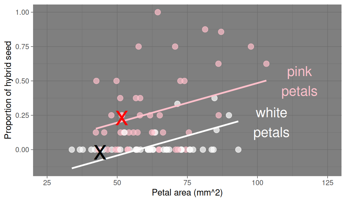
library(broom)
lm(prop_hybrid ~ petal_color + petal_area_mm, data = gc_rils)            |>
    augment()                                                            |>
    ggplot(aes(x = petal_area_mm, y = prop_hybrid, color = petal_color))  +
    geom_point()                                                          +
    geom_smooth(aes(y = .fitted))

Scatterplot showing proportion of hybrid seeds as a function of petal area for Clarkia parviflora RILs. Points are colored by petal color. A fitted linear trendline with the same slope for each petal color is shown, matching the general linear model. Individual plants $i=1$ and $i=3$ are emphasized with black and red Xs, respectively. The plot allows hovering for more information. — Figure 1: **Proportion of hybrid seeds as a function of petal area and petal color in parviflora RILs.** This plot shows both the data (points) and model predictions (lines). By default, geom_smooth() fits separate slopes for each petal color - but our model has a single slope. Check out the code above to see how to make the lines match our actual model. Individuals $i=1$ and $i=3$ are highlighted with black and red Xs, respectively.

Conditional means from General linear Models

With the estimates above, we can return to our general linear model equation to find conditional means: \[\widehat{\text{Prop hybrids}}_i = b_0 + b_1 \times \text{PETAL AREA}_i + b_2 \times \text{WHITE}_i\] \[\widehat{\text{Prop hybrids}}_i = -0.0894 + 0.00576 \times \text{PETAL AREA}_i - 0.244192 \times \text{WHITE}_i\]

i	petal_area_mm	petal_color	prop_hybrid
1	43.9522	white	0.000
2	55.7863	pink	0.125
3	51.7031	pink	0.250
4	57.2810	white	0.000

A worked example and challenge questions

The table below shows values of the explanatory and response variables for the first four samples in the gc_rils dataset. Individuals $i = 1$ and $i = 3$ are shown in black and red x’s in Figure 1, and I provide R code for calculating the prediction and residual for individual $i=1$ below.

# prediction for i = 1
# prediction = intercept + slope * petal area + effect of white * white (1) or pink(0)
y_1_pred <- -0.0894 + 5.76e-3 * 44 - 0.244 * 1       

### The prediction for individual 1 is
y_1_pred

[1] -0.07996

# Residual equals observation minus prediction 
# So the residual for individual 1 is (the observed value is 0, from the table above)
0 - y_1_pred

[1] 0.07996

In the webR session below:

Find the predicted proportion of hybrid seed for individual $i=3$ .
Find the residual of for individual $i=3$ .

# Prediction for i = 3
# b0   + b1 * petal area + b2 * white
-0.0894 + 5.76e-3 * 51.7 #   no b2 because its pink

[1] 0.208392

# Residual for ind i = 3
0.25  - (-0.0894 + 5.76e-3 * 51.7)

[1] 0.041608

Residual Sum of Squares & $SS_\text{resid}$

Again we can calculate the sum of squared residuals, and the residual standard deviation. Either with the augment() output:

lm(prop_hybrid ~ petal_area_mm + petal_color, data = gc_rils)  |>
  augment()                                                    |>
  mutate(sq_resid=.resid^2)                                    |>
  summarise(SS_resid = sum(sq_resid), 
            n        = n(),
            sd_resid = sqrt(SS_resid / (n - 3))) # three parameters to estimate

# A tibble: 1 × 3
  SS_resid     n sd_resid
     <dbl> <int>    <dbl>
1     3.38    89    0.198

Or more simply with the sigma() function:

lm(prop_hybrid ~ petal_area_mm + petal_color, data = gc_rils)         |>
  sigma()

[1] 0.1982151

Conclusion: Including petal area and petal color in the model reduced the residual standard deviation substantially! Compared to a “mean only” model a model including petal color and area reduced the residual standard deviation by about 16% – dropping from 0.237 to 0.198.

Wrapping Up: Two Predictors, One Model

Above, we extended a simple linear model to include two predictors — one continuous and one categorical. We could, of course, have had two categorical predictors, two numeric predictors, or more than two predictors as well, even interactions between predictors. By adding multiple predictors, we can better account for biological complexity — modeling how several traits simultaneously influence a response.

General Linear models in R

Conditional means from General linear Models

A worked example and challenge questions

Residual Sum of Squares & \(SS_\text{resid}\)

Wrapping Up: Two Predictors, One Model