library(dplyr)
library(readr)
library(tidyr)
library(conflicted)
conflict_prefer(name = "select", winner = "dplyr")

path <- "https://raw.githubusercontent.com/ybrandvain/datasets/refs/heads/master/clarkia_rils.csv"
ril_data <- read_csv(path)• 4. Checking Data Review
Motivating scenario: you have your data loaded into R and want to examine it and prepare for analysis.
Learning goals: By the end of this sub-chapter you should be able to
- Use
dplyr’sglimpse()to get a sense of our data.
- Use
dplyr’sselect()function to limit our data to a few variables of interest.
- Use
dplyr’srename()` function to change the names of specific columns.
NOTE: This is largely a review and consolidation of material from the previous chapter.
The good news is that R has many functions to help us deal with data. The bad news is that this means that there are a lot of R functions to keep in mind when dealing with data. So we begin this section with a review of three skills we learned in the previous chapter:
- Peeking at our data with
dplyr’sglimpse()function to know the names of each column and the type of data in each.
- Choosing columns of interest with
dplyr’sselect()function. This let’s us focus on a few columns of interest.
- Changing the names of a few columns with
dplyr’srename()function to make the data easier to wrangle.
To set up this work we load libraries and data:
A glimpse() at our data.
To deal with data you must know how to refer to it and what type of data it is. The glimpse() function provides information on both accounts:
glimpse(ril_data)Rows: 593
Columns: 17
$ ril <chr> "A1", "A100", "A102", "A104", "A106", "A107", "A10…
$ location <chr> "GC", "GC", "GC", "GC", "GC", "GC", "GC", "GC", "G…
$ prop_hybrid <dbl> 0.000, 0.125, 0.250, 0.000, 0.000, 0.125, NA, 0.00…
$ mean_visits <dbl> 0.0000, 0.1875, 0.2500, 0.0000, 0.0000, 0.0000, NA…
$ growth_rate <chr> "1.272", "1.448", "1.8O", "0.816", "0.728", "1.764…
$ petal_color <chr> "white", "pink", "pink", "white", "white", "pink",…
$ petal_area_mm <dbl> 43.95220, 55.78633, 51.70312, 57.28095, 68.55464, …
$ date_first_flw <dbl> 95.38681, 96.75742, 97.95671, 95.21548, 96.75742, …
$ node_first_flw <dbl> 20.51416, 25.26508, 24.91316, 15.58727, 18.40264, …
$ petal_perim_mm <dbl> 43.07237, 43.84228, 47.29937, 47.01340, 55.71933, …
$ asd_mm <dbl> 0.4466794, 1.0730412, 0.6744473, 0.9591572, 1.4146…
$ protandry <dbl> 1.2812553, 1.1107347, 0.9402142, 1.2812553, 2.8159…
$ stem_dia_mm <dbl> 1.924, 2.328, 2.422, 1.826, 1.890, 1.954, 2.120, 1…
$ lwc <dbl> 0.8311, 0.8376, 0.8421, 0.8236, 0.8249, 0.8316, 0.…
$ crossDir <chr> "A", "A", "A", "A", "A", "A", NA, "A", "A", "A", "…
$ num_hybrid <dbl> 0, 1, 2, 0, 0, 1, NA, 0, 0, 2, 0, NA, NA, 1, 0, NA…
$ offspring_genotyped <dbl> 8, 8, 8, 8, 8, 8, NA, 8, 8, 8, 8, NA, NA, 8, 8, NA…Also remember that:
- The
View()function opens up the entire datasheet in a new window.
janitor’sclean_names()function standardizes and improves column names.
select()ing columns of interest
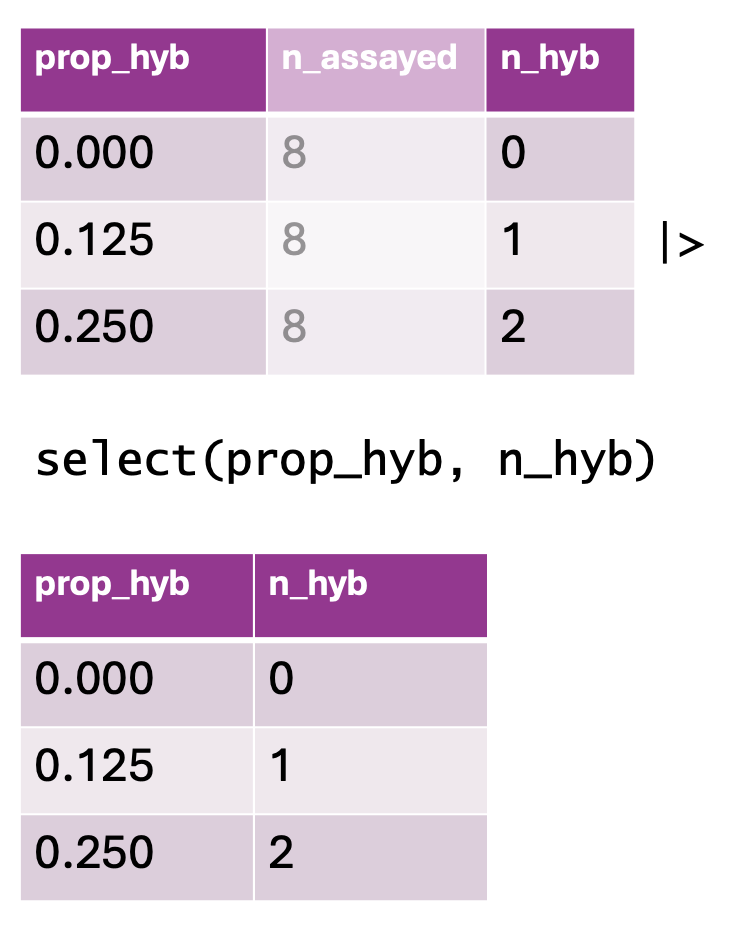
select() function to retain specific columns from a dataset. The top table contains three columns: prop_hyb (proportion of hybrids), n_assayed (number of individuals assayed), and n_hyb (the computed number of hybrids). The select(prop_hyb, n_hyb) function is applied, keeping only the prop_hyb and n_hyb columns. The bottom table displays the resulting dataset after column selection.
The dataset above is not tiny – seventeen columns accompany the 593 rows of data. To simplify your life, use dplyr’s select() function to limit the variables of interest:
location: The plant’s location. The pollinator visitation experiment was limited to two locations (eitherSRorGC), while the hybrid seed formation study was replicated at four locations (SR,GC,LBorUS). This should be a<chr>(character), and it is!prop_hybrid: The proportion of genotyped seeds that were hybrids.
mean_visits: The mean number of pollinator visits recorded (per fifteen minute pollinator observation) for that RIL genotype at that site. This should be a number<dbl>(double), and it is.petal_area_mm: The area of the petals (in mm). This should be a number<dbl>(double), and it is!
asd_mm: The distance between anther (the place where pollen comes from) and stigma (the place that pollen goes to) on a flower. The smaller this number, the easier it is for a plant to pollinated itself. This should be a number<dbl>(double), and it is.
growth_rate: This should be a number but is a <chr> character. We will address why this is a problem and how to fix it in the next sub-section.
ril_data |>
  select(location,   prop_hybrid,  mean_visits, petal_color,
         petal_area_mm,  asd_mm, growth_rate)
# A tibble: 593 × 7
location prop_hybrid mean_visits petal_color petal_area_mm asd_mm growth_rate
<chr> <dbl> <dbl> <chr> <dbl> <dbl> <chr>
1 GC 0 0 white 44.0 0.447 1.272
2 GC 0.125 0.188 pink 55.8 1.07 1.448
3 GC 0.25 0.25 pink 51.7 0.674 1.8O
4 GC 0 0 white 57.3 0.959 0.816
5 GC 0 0 white 68.6 1.41 0.728
6 GC 0.125 0 pink 66.3 0.788 1.764
7 GC NA NA <NA> 51.5 0.6 1.584
8 GC 0 0 white 48.1 0.561 1.476
9 GC 0 NA white 51.6 1.02 1.144
10 GC 0.25 0 white 89.8 0.618 1
# ℹ 583 more rowsrename()`ing columns of interest
Recall that we can change column names to be more descriptive or less elaborate with dplyr’s rename()` function:
ril_data |>
  select(location,  prop_hybrid,  mean_visits, petal_color,
         petal_area_mm, asd_mm, growth_rate) |>
  rename(petal_area = petal_area_mm,
         asd        = asd_mm,
         visits = mean_visits)
# A tibble: 593 × 7
location prop_hybrid visits petal_color petal_area asd growth_rate
<chr> <dbl> <dbl> <chr> <dbl> <dbl> <chr>
1 GC 0 0 white 44.0 0.447 1.272
2 GC 0.125 0.188 pink 55.8 1.07 1.448
3 GC 0.25 0.25 pink 51.7 0.674 1.8O
4 GC 0 0 white 57.3 0.959 0.816
5 GC 0 0 white 68.6 1.41 0.728
6 GC 0.125 0 pink 66.3 0.788 1.764
7 GC NA NA <NA> 51.5 0.6 1.584
8 GC 0 0 white 48.1 0.561 1.476
9 GC 0 NA white 51.6 1.02 1.144
10 GC 0.25 0 white 89.8 0.618 1
# ℹ 583 more rowsGotcha’s and warnings:
Warning: R doesn’t remember changes until you assign them.
I like to test my code before overwriting the old data with the new. So, now that we see that our code worked as expected, enter the following. Otherwise ril_data is unchanged
ril_data <- ril_data |>
  select(location,  prop_hybrid,  mean_visits, petal_color,
         petal_area_mm, asd_mm, growth_rate) |>
  rename(petal_area = petal_area_mm,
         asd        = asd_mm,
         visits     = mean_visits)
Warning: Consider order
Remember: once you rename a column, the old name no longer exists in the pipeline. With this in mind consider the code below. Which code will work?
Feel free to mess around in the webR environment below (data and packages are loaded for you) to see for yourself.
# A)
ril_data |>
  select(location,  prop_hybrid,
         mean_visits, petal_color,
         petal_area_mm, asd_mm, growth_rate) |>
  rename(petal_area = petal_area_mm,
         asd        = asd_mm,
         visits     = mean_visits)

# B)
ril_data |>
  rename(petal_area = petal_area_mm,
         asd        = asd_mm,
         visits     = mean_visits) |>
  select(location,  prop_hybrid,
         mean_visits, petal_color,
         petal_area_mm, asd_mm, growth_rate)

# C)
ril_data |>
  rename(petal_area = petal_area_mm,
         asd        = asd_mm,
         visits     = mean_visits) |>
  select(location,  prop_hybrid,
         visits, petal_color, petal_area,
         asd_mm, growth_rate)