• 15. Uncertain-2t

Motivating scenario: We have summarized the difference in means of two groups. But we know that all estimates should be accompanied by an estimate of their uncertainty.

Learning goals: By the end of this section, you should be able to:

• Quantify uncertainty in estimates of difference in means using the:
  • Standard Error.
    
  • The 95% Confidence Interval.
    

ril_link <- "https://raw.githubusercontent.com/ybrandvain/datasets/refs/heads/master/clarkia_rils.csv"
SR_visits <- readr::read_csv(ril_link) |>
    dplyr::rename(visits = mean_visits)  |>
    dplyr::filter(location == "SR",
                  !is.na(petal_color),
                  !is.na(visits))        |>
    dplyr::select(petal_color, visits)

color_visit_summaries <- SR_visits |>
  group_by(petal_color)|>
  summarise(MEAN  = mean(visits),
            VAR   = var(visits),
            N     = n())

---

Estimating uncertainty in the mean difference

A “point” estimate is just that – our informed guess of a parameter value. Point estimates come from samples, so we should always pair them with an estimate of uncertainty. For the difference in means, we quantify uncertainty from the “pooled standard error” and use this with the t-distribution to generate a confidence interval.

Remember: The equation for the pooled variance: \[s^2_p = \frac{\text{df}_1 \times s_1^2+ \text{df}_2 \times s_2^2}{\text{df}_\text{total}}\] So in our example: \[s^2_p = \frac{56 \times 2.71+ 49 \times 0.833}{56+49}\] \[s^2_p = 1.834\].

• \(s_i^2\): The variance within group \(i\).
  
• \(\text{df}_i\): The degrees of freedom in group \(i\).
  
• \(\text{df}_\text{total}\): The total degrees of freedom (defined in text below).

---

\(SE_{\overline{x_1}-\overline{x_2}}\) for our example:

\[ \begin{align} SE_{\overline{x_1}-\overline{x_2}} &= \sqrt{s_p^2 \Big(\frac{1}{n_1} + \frac{1}{n_2}\Big)}\\ &= \sqrt{1.834\times\Big({\frac{1}{57}+\frac{1}{50}\Big)}}\\ &=0.2624 \end{align} \]

• The standard error for the difference in means is a strange looking equation. Recall that \(s^2_p\) is the “pooled variance” and using this value implies that we believe that variance is similar within each group:

\[SE_{\overline{x_1}-\overline{x_2}} = \sqrt{s_p^2 \Big(\frac{1}{n_1} + \frac{1}{n_2}\Big)}\]

• The 95% confidence interval of the difference in means. This is pretty straightforward. Now that we have our standard error, we simply multiply it by \(t_{\text{crit, }{\alpha=0.05\text{, }df_\text{total}}}\).

  • The total degrees of freedom is the sum of the degrees of freedom for each estimate:

\[ \begin{align} df_\text{total} &= df_1+df_2 \\ &= (n_1 - 1) + (n_2-1)\\ &= n_{total}-2 \end{align} \]

Let’s calculate the standard error and 95% confidence interval for the estimate of the mean difference “by hand” in R:

thing	value
mean_diff	1.026
pooled_var	1.834
df_total	105.000
se	0.262
crit_t	1.983
lower_95_CI	0.505
upper_95_CI	1.546

color_visit_summaries|>
  mutate(DF = N-1)|>
  summarise(mean_diff   = diff(MEAN) |> abs(),
            pooled_var  = sum((N-1)*(VAR)) / (sum(N)-2),
            df_total    = sum(DF),
            se          = sqrt(pooled_var*(sum(1/N))),
            crit_t      = qt(p = 0.025, 
                             df = df_total, 
                             lower.tail = FALSE),
            lower_95_CI = mean_diff - se * crit_t,
            upper_95_CI = mean_diff + se * crit_t)

We have done all our calculations on the linear scale, not the log(x+0.2) transformed data. That is because the data were close enough to meeting assumptions. If we decided to analyze data on a transformed scale, we would need to communicate these results to our audience in a way they could understand.

A complement: Bootstrap to quantify uncertainty

Recall that bootstrapping approximates the sampling distribution by resampling the data with replacement. See the section on uncertainty for review.

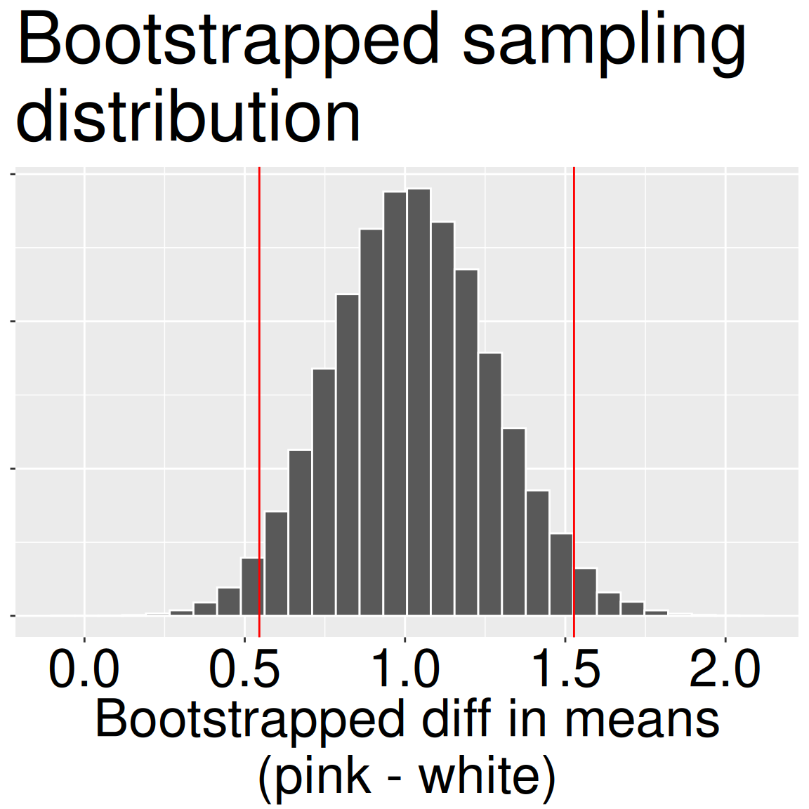
Because our data did not perfectly conform to the assumptions of our statistical procedure, we cannot be sure that the results from our analysis are valid. To evaluate the robustness of my conclusions, I bootstrap the data to obtain a 95% confidence interval without making assumptions about equal variance or normality. The 95% bootstrap CI ranges from 0.54 to 1.53. This interval is roughly the 95% confidence interval from 0.50 to 1.546 found by the two-sample t-test. This demonstrates that our statistical conclusions are robust to the violations of the assumptions of normality and equal variance in the data.

In a later section you will see that this is basically what we would get from a version of the t-test that does not assume equal variance. This is all to say that we need not be too worried about the violation of assumptions in this case.

As we found in this case, the t can be quite robust to violations of assumptions. This does not mean we should ignore these violations. Rather, it means that when we violate assumptions we should put on our thinking caps, and subject our conclusions to another round of scrutiny.

Figure 1: Bootstrap sampling distribution of the difference in mean visits (pink − white). The histogram shows 50,000 bootstrapped estimates of the mean difference; the red vertical lines mark the 95% percentile CI (here ≈ 0.50 to 1.52).

Bootstrapped SEs and CIs

se	lower_95	estimate	upper_95
0.251	0.546	1.026	1.527

library(infer)

# SUMMARIZE THE DATA
raw_diff <- SR_rils %>%
  specify(mean_visits ~ petal_color) |>            # response ~ explanatory
  calculate(stat = "diff in means",                # difference in group means
            order = c("pink", "white"))

# BOOTSTRAP
boot_SR_visits <-  SR_rils %>%
  specify(mean_visits ~ petal_color) |>            # specify response ~ explanatory
  generate(reps = 5000, type = "bootstrap") |>     # resample
  calculate(stat = "diff in means",                # calculate difference in means
            order = c("pink", "white"))

# SUMMARIZE THE BOOTSTRAP
bootsummary <- boot_SR_visits |>
  summarise(
    se = sd(stat),
    lower_95 = quantile(stat, prob = 0.025),
    estimate = pull(raw_diff ),
    upper_95 = quantile(stat, prob = 0.975)
    )