Motivating example: We have numerous explanatory variables and we want to build a multiple regression model. But before we get carried away in interpreting our results we want to know if our results can even be trusted.
Learning goals: By the end of this section, you should be able to:
Explain why multiple regression can struggle when explanatory variables are strongly correlated with one another.
Use variance inflation factors (VIFs) to diagnose multicollinearity.
Use diagnostic plots to evaluate residual normality and unequal variance.
Assumptions of multiple regression
Multiple regression includes the same general assumptions as other standard linear models. But before refreshing those, let’s introduce the new assumption of multiple regression:
No multicollinearity: Multiple regression assumes that explanatory variables are not very strongly correlated. If they are too strongly correlated, estimates get wobbly.
OK back to the standard linear model assumptions, with a few details about their application / detection in multiple regression:
Unbiased data collection: The data were collected in a way that lets us answer the biological question without systematic bias.
Independence: Observations, and therefore residuals, are independent of one another after accounting for the predictors in the model.
Linearity: The model describes the expected value of the response by adding up components of the model. For a multiple regression this means that we assume we can make reasonable predictions by adding the contributions of each explanatory variable in our model.
Normality of residuals: The residuals are approximately normally distributed. As in linear regression, we evaluate the normality of residuals \(e_i\) with diagnostic plots.
Homoscedasticity: The variance of residuals is roughly constant across fitted values, \(\hat{Y}_i\). Again this is best evaluated with a diagnostic plot.
Multiple regression assumes no multicollinearity
This does not mean that explanatory variables must be completely uncorrelated. In fact, a major strength of multiple regression is that it allows us to “adjust” for associations among explanatory variables. The problem arises when the association between variables is so strong that it becomes difficult to estimate their separate contributions. If two explanatory variables are super strongly associated, the model has relatively little information about what happens when one changes while the other stays constant. As a result, coefficients can become unstable, standard errors get big, and interpreting what ‘adjustment’ means gets tricky.
As a rough rule of thumb, we don’t worry much about associations between explanatory variables with a correlation coefficient less than 0.8. A more formal diagnostic is the “variance inflation factor” (VIF). A VIF asks how much the uncertainty in a coefficient is inflated because that predictor is correlated with the other predictors in the model. When VIFs get to about five we might worry a bit. When they get above ten, this becomes even more concerning.
The vif() function in the car package calculates variance inflation factors for each variable in a model.
If your model includes a categorical explanatory variable with more than two categories, you will get GVIFs which aim to calculate something like a VIF for such models. In that case, pay attention to the GVIF^(1/(2*Df)) value.
You can see that we need not worry at all about multicollinearity in our model. But, if we did, there are numerous potential solutions to multicollinearity – you can either drop a variable highly correlated with another, or take some form of averaging or dimensionality reduction (e.g. PCA) to reduce this issue.
Evaluating other assumptions
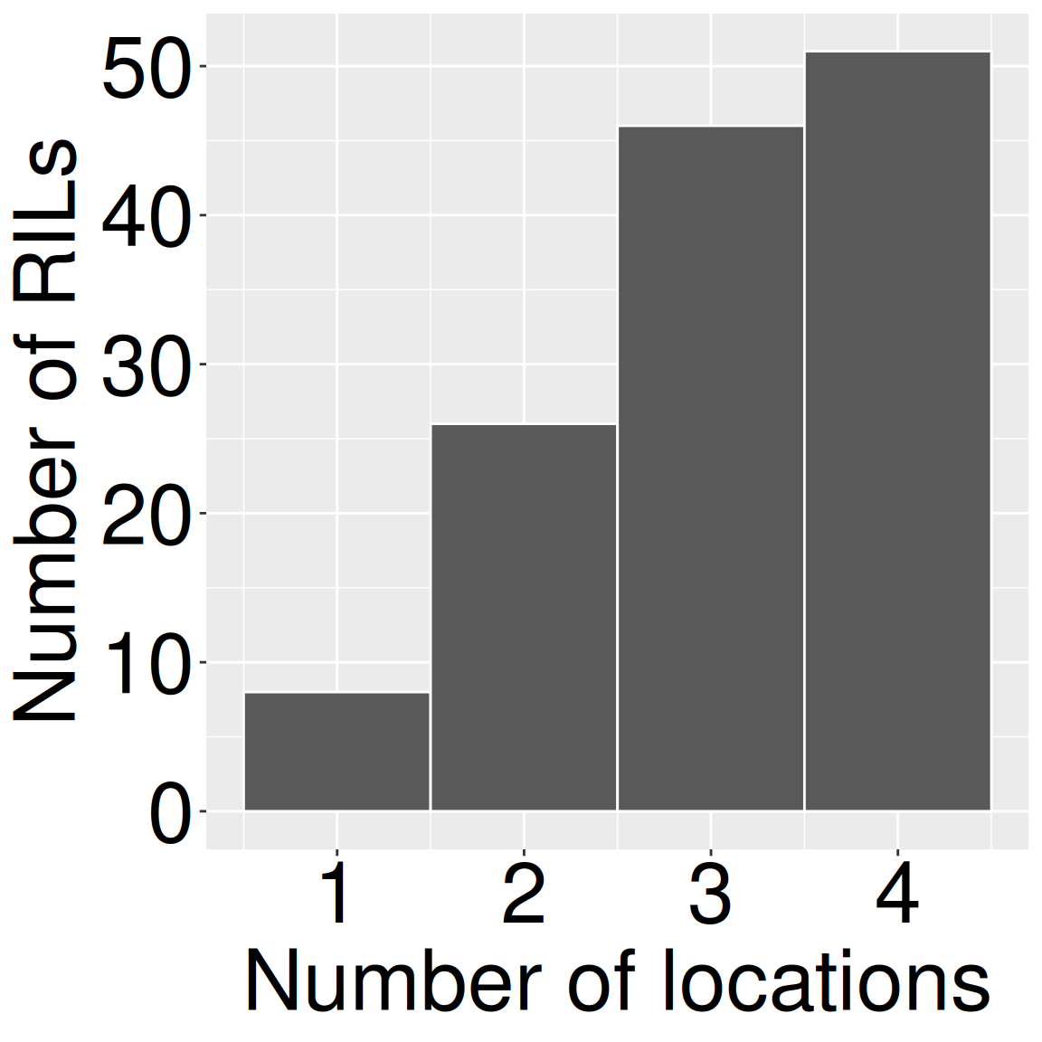
Data are not independent. In most cases we planted the same RIL at three or four locations (Figure 1). Because observations from the same RIL may be more similar to each other than observations from different RILs for many reasons, the data are not independent.
Figure 1: Number of locations represented for each RIL. Most RILs were measured at three or four locations, meaning rows in the data set are not fully independent.
This is a problem because the model treats each row as a separate piece of information. If the same RIL appears several times, then those rows are not really separate in the same way that rows from different RILs are separate. As a result, our model may act more confident than it should: standard errors may be too small, confidence intervals may be too narrow, and p-values may be too optimistic.
We have a few options here:
We could average each RIL across locations. Such averaging would remove non-independence as we would only have one data point per RIL, While this approach is sometimes reasonable, at best it also throws away information about location. In this case, it’s got another issue - because not all RILs were planted at all locations, the unmodeled influence of location could influence our results.
We could include RIL in the model. When we come to “mixed effect models” we will see the proper way to do this. However, this is an advanced technique that goes beyond our current knowledge, and putting the 100+ RILs in our model as a “fixed effect” is a bad idea. This is because RILS come with petal color, petal area, and ASD, so including a separate coefficient for every RIL would eat up all the among RIL variation needed to estimate the effects of the explanatory variables we care about.
So, for now, we will:
Move on while pointing out this non-independence We will remember to point out that our p-values and standard errors are smaller than they should be. But this is a pretty good start. Better to start and do something imperfect, and be honest, than lying or doing nothing.
Residuals are not perfectly normal, and the response is bounded
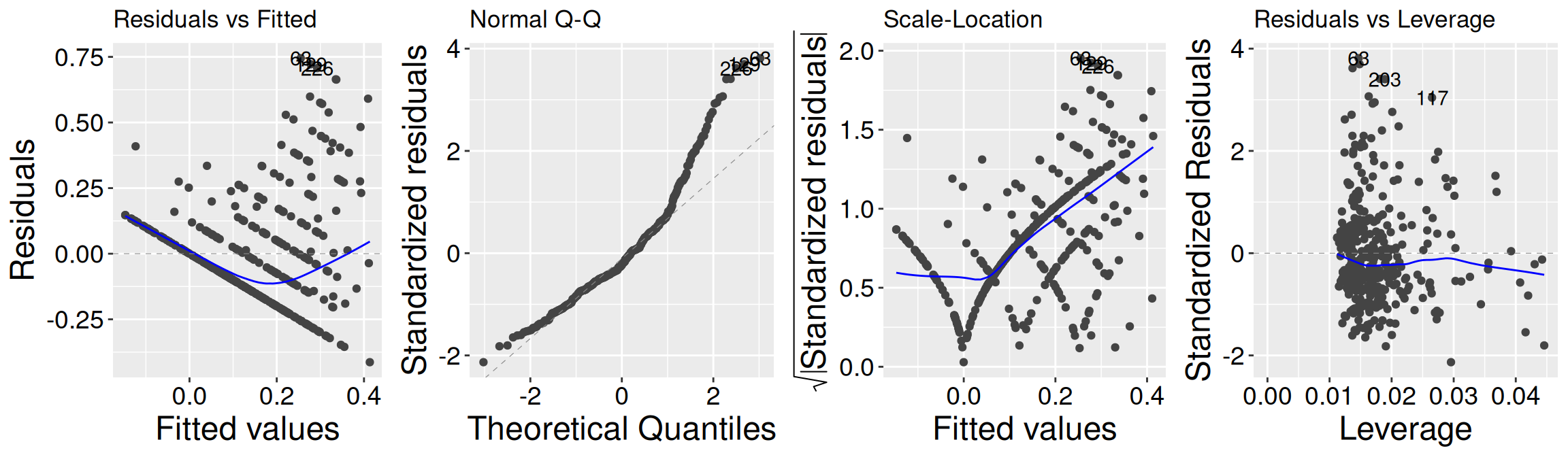
The diagnostic plots in ?fig-diag are clearly weird. For example, we see weird lines in the residual vs. fitted plot, and strange “V” shapes in the scale location plot. We also see a modest increase in very large values in the QQ-plot.
These issues all come from the same basic truth of our data – it is not normal, but rather is “binomial.” Each seed is either a hybrid or not, and we measure a modest number (usually eight, but sometimes fewer) seeds per mom. Thus our data and the residuals CANNOT be normal.
Later, you may learn about logistic regression, a generalized linear model built for binomial data. But, for now, we can note that although the shapes and patterns in the diagnostic plots are weird, and the data are clearly not perfectly normal, the deviations are not so extreme as to call our results into question. Thus, for now we go on with our standard multiple regression approach!
As you have seen, I pointed out several ways in which our data do not fully meet the assumptions of standard multiple regression, but I nevertheless suggested that we continue with that approach. I made this choice for an important reason:
Avoid analysis paralysis. Statistics can feel overwhelming, especially when students come to believe that every analysis has one uniquely correct form and that anything less is simply wrong. That way of thinking is rarely helpful. A simpler, imperfect analysis can often provide a useful starting point, especially when its limitations are clearly acknowledged. Simpler approaches are also usually easier to understand, evaluate, and communicate than more sophisticated ones. My goal is therefore to help you begin with a reasonable analysis rather than become paralyzed while searching for a perfect one. See this short paper for more.
That said, some methods are better suited to particular data structures than standard multiple regression. In this case, a generalized linear mixed-effects model would better account for both the binomial response and the repeated measurements of each RIL. Even then, however, we must weigh improved statistical fit against added model complexity and the challenges of explaining and communicating the analysis. The goal is not statistical purity, but an analysis that is appropriate, understandable, and honest about its limitations.