hybrid_anova <- lm(admix_proportion ~ site, data = clarkia_hz)• 17. ANOVA is a linear model
Motivating Scenario: You know that many statistical models are simply a type of linear model. How can we think about an ANOVA as a linear model and interpret the coefficients from this model?
Learning Goals: By the end of this subchapter, you should be able to:
Recognize that ANOVA is a special case of a linear model.
Interpret model coefficients (intercept, slopes) in the context of group means.
Know what a residual is and calculate residuals
Change the reference level and interpret how it affects model output.
Setting up our linear model
Recall that “linear models” are “linear” because we find an individual’s predicted value \(\hat{Y_i}\) by adding up predictions from each component of the model. So, for example, \(\hat{Y_i}\) equals the parameter estimate for the “intercept”, \(a\), plus its value for the first explanatory variable, \(x_{1,i}\), times the effect of this variable, \(b_1\), plus its value for the second explanatory variable, \(x_{2,i}\), times its effect, \(b_2\), etc.
\[\hat{Y}_i = a + b_1 x_{1,i} + b_2 x_{2,i} + \dots{}\]
Just like a one- or two-sample t-test, the ANOVA is a linear model. As such, it models group means as a function of group membership. This works by:
picking one group as the “reference level” and having that group’s mean represented as the intercept. Then each “slope” \(b\) is the difference between that group’s mean and the reference group’s mean, and the corresponding \(x_i\)s are one if the individual is in that group and zero otherwise.
By default R chooses the reference levels as the alphabetically first one. We often don’t want that (e.g. you may want the control to be first). The fct_relevel() function in the forcats package can help (see fyi below)!
(Intercept)     siteS22      siteSM      siteS6
     0.0071      0.0183      0.0025      0.0221
We cast this as a linear model as follows: \(\widehat{\text{admix prop}}_i = 0.0071 + 0.0183 \times \text{S22}_{i} + 0.0025 \times \text{SM}_{i} + 0.0221 \times \text{S6}_{i}\).
Here SR is the “reference level”, so:
- SR’s mean admixture proportion equals the intercept, 0.0071.
- S22’s mean admixture proportion equals 0.0254. This represents the intercept, 0.0071, plus the term for S22, 0.0183.
Practice
Use the linear model output to find the estimated admixture proportion at each of the following locations:
Have a try!
- Squirrel Mountain (SM) .
- Site 6 (S6) .
Residuals
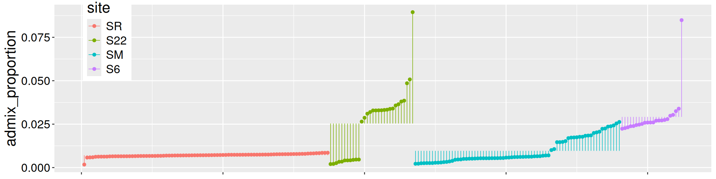
Of course, individual observations deviate from their predicted value. As you now know, the residual, \(e_i\), describes the difference between an observation, \(Y_i\), and its predicted value, \(\hat{Y_i}\). Figure 1 shows the residuals as the length of the lines connecting individual observations to group means.
Mathematical descriptions of residuals
\[e_i=Y_i - \hat{Y_i}\]
\[Y_i=\hat{Y_i}+e_i\]
Recall that broom’s augment() function in the broom package shows \(\hat{Y_i}\) as the .fitted column, and the residuals as the .resid column:
library(broom)
augment(hybrid_anova)| admix_proportion | site | .fitted | .resid |
|---|---|---|---|
| 0.0265 | S22 | 0.0254 | 0.0011 |
| 0.0329 | S22 | 0.0254 | 0.0075 |
| 0.0895 | S22 | 0.0254 | 0.0641 |
| 0.0042 | S22 | 0.0254 | -0.0212 |
| 0.0041 | S22 | 0.0254 | -0.0212 |
| 0.0033 | S22 | 0.0254 | -0.0221 |
R assigns reference levels in alphabetical order. This does not necessarily reflect our biological understanding or experimental design.
Changing reference levels
Alphabetical order is not always the “right” order. For example, the analysis below compares plant growth (measured as biomass) in a control environment to hot or cold treatments (group).
lm(biomass ~ group, data = plant_growth)
Call:
lm(formula = biomass ~ group, data = plant_growth)

Coefficients:
 (Intercept)  groupcontrol     groupwarm
       4.661         0.371         0.865
In this case, it makes the most sense to use “control” as the reference level and to express treatment effects as deviations from the control. However, alphabetically, “cold” comes before “control,” so “cold” is used as the reference level by default. Changing the reference level will not affect our statistical conclusions, but it can make the model output and interpretation easier to present and discuss.
The fct_relevel() function in the forcats package makes changing the reference level straightforward:
# Replace data with the name of the data object
# Replace x with the name of the explanatory variable
# Replace "<REF LEVEL>" with the name of the reference level

data <- data |>
  mutate(x = fct_relevel(x, "<REF LEVEL>"))
Now you try! Changing the reference level of group to control in the plant_growth data. Then run the relevant linear model.
# load packages:
library(dplyr)
library(forcats)

# Change reference level
plant_growth <- plant_growth |>
  mutate(group = fct_relevel(group, "control"))

# Run the linear model
lm(biomass ~ group, data = plant_growth)
Call:
lm(formula = biomass ~ group, data = plant_growth)

Coefficients:
(Intercept)    groupcold    groupwarm
      5.032       -0.371        0.494
As you can see from your work (or my answer), we have changed the reference level: our model now includes the terms (Intercept), groupcold, and groupwarm!
Have a try!
Practice From the output above, we see the mean biomass in the control is (write -99 for NA): .
Practice. In the new model, the value 0.494 represents:.
Practice. Compared to the initial model, this new version:.