Motivating Scenario: In the previous chapter, we asked whether two groups differed. But we often work with more than two categories. How do we deal with these cases? We could compare every pair of sites using t-tests—but this quickly leads to a problem. As we run more tests, we increase our chances of finding differences just by chance. So how do we test for differences across many groups without fooling ourselves?
Learning Goals: By the end of this chapter, you should be able to:
Explain why multiple pairwise t-tests lead to inflated false positive rates.
Use ANOVA to test the null hypothesis that all group means are equal.
Interpret the F statistic in the context of comparing more than two groups.
Apply post-hoc tests to identify which groups differ, while accounting for multiple testing.
We have considered both the two-sample t-test, and the variance partitioning approach, to test the null hypothesis that group means are equal. We saw that these approaches give the same answers when analyzing a continuous response variable with a binary explanatory variable. Here, we consider what to do when our explanatory variable has more than two “levels”.
We will see that testing for a difference between each group mean in a pairwise manner introduces a “multiple testing problem.” The multiple testing problem simply means that the probability of rejecting one or more true null hypotheses increases as you test more null hypotheses.
We show that the ANOVA approach allows us to overcome this multiple testing problem by testing a single null hypothesis – that the true group means are identical (i.e. there is no among-group variance in the population). We then show how you can use the “post-hoc” testing framework to adjust your p-values (or other means to appropriate calibrate the \(\alpha\) thresholds) to incorporate the fact that you are testing multiple hypotheses after finding that not all group means are equal.
Example data
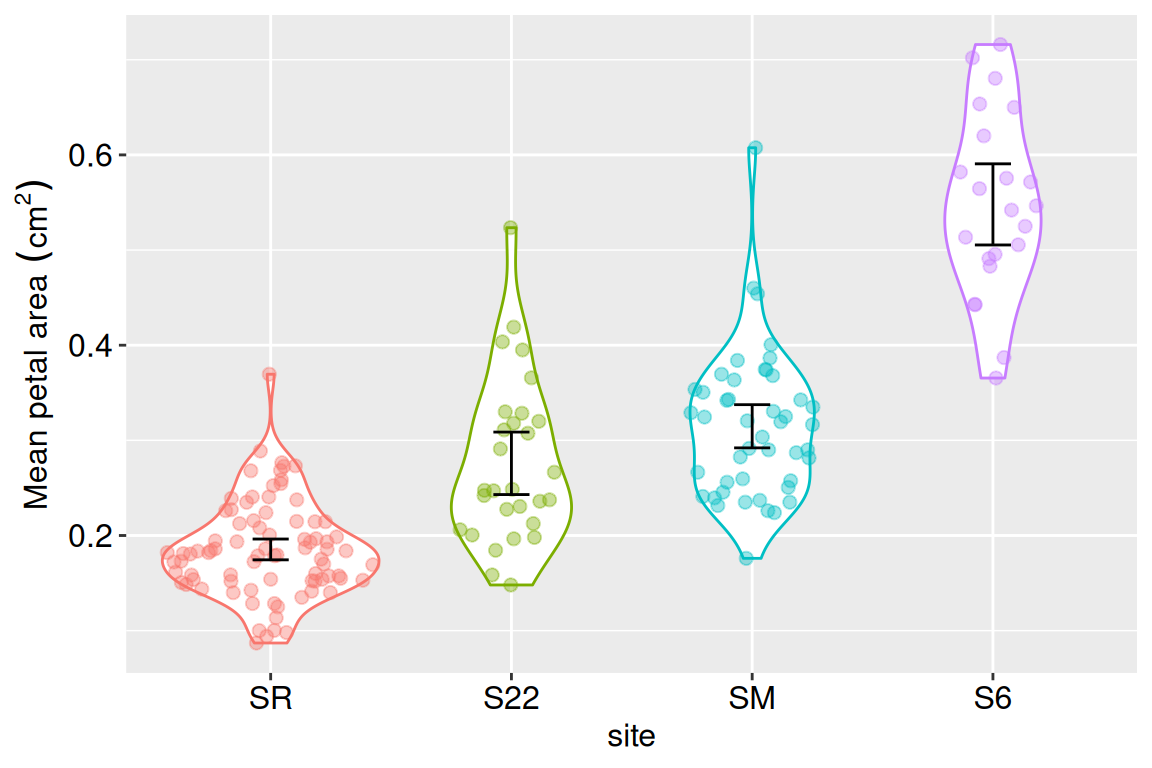
We will revisit the data from parviflora plants in natural hybrid zones introduced in the previous chapter. This time, we will look at the variability in petal area among parviflora populations. This is potentially interesting because ecological features and the admixture proportion differ across sites, and it’s worth noting whether this is associated with any differences in key phenotypes in the field! The data are plotted below:
Code for plotting
library(ggforce)ggplot(clarkia_hz , aes(x = site, y =mean_petal_area_sq_cm, color = site))+geom_violin()+geom_sina(alpha = .4, size =2)+stat_summary(fun.data ="mean_cl_normal",geom ="errorbar", color ="black",width = .15)+labs(y =expression(Mean~petal~area~(cm^2)))+theme(legend.position ="none", axis.text =element_text(size =12), axis.title =element_text(size =12))
Let’s goooooo
So how can we analyze these data? As we will see soon, doing a bunch of t-tests is not the answer, but an ANOVA followed by post-hoc tests is! Let’s see why this is, and how to do it.