Motivating scenario: We fit a model with an interaction, and this interaction seems to influence our predictions. Now we want to test the null hypothesis that the interaction (and main effects) reflect only sampling error from one population rather than a real difference among populations.
Learning goals: By the end of this section, you should be able to:
State the null hypothesis associated with an interaction term.
Use a Type II ANOVA table to test an interaction as a whole.
Evaluate whether the data provide adequate overlap for estimating an interaction.
Apply standard linear-model diagnostic checks to a model containing an interaction.
We found that the slopes describing the increase in the proportion of hybrid seeds in white- and pink-petaled RILs looked very different. The increase in white-petaled RILs was subtle, while the increase in pink-petaled RILs looked obvious. But, we know that we cannot always trust our eyes, and that we can mistake noise for signal. So, here I show how to test the statistical significance of the terms in such models.
model <-lm(prop_hybrid ~ petal_area_mm + petal_color + petal_area_mm:petal_color , data = rils)
In the model of the proportion of hybrid seeds as a function of petal area, petal color and their interaction (above), there are three terms. Each term comes with a null hypothesis we are testing.
The term petal_area_mm is associated with the null hypothesis that the slope is zero (after adjusting for petal color).
The term petal_color is associated with the null hypothesis that the mean proportion of hybrid seeds of pink- and white-petaled RILs are equal (after adjusting for petal area).
The term petal_color:petal_area_mm is associated with the null hypothesis that slopes do not differ between white- and pink-petaled RILs.
Here I suggest using Type II sums of squares. In Type II sums of squares, we test each main effect after “adjusting” for the others, and we test each interaction effect after adjusting for the main effects and all other interaction effects of the same order.
You may sometimes see people (or computer programs) use Type III sums of squares. Type III sums of squares test each term after adjusting for all other terms in the model, including interactions. The type III approach tests slightly different null hypotheses which I find harder to think about and present.
Testing the nulls
As in our introduction to multiple regression, we do not use the anova() function to test the null, because it conducts Type I sums of squares. We also do not use the summary() or tidy() functions, as the p-values in that output describe the deviation of model coefficients from zero, rather than the nulls stated above. Instead, we use the Anova() function in the car package:
We resoundingly reject all three null hypotheses. But what does this mean? Well, rejecting the null of no interaction is relatively easy to explain – we reject the null that slopes are the same for white- and pink-petaled RILs. The interpretation of results for the main effects is more complex, as the meaning of main effects can change in the presence of an interaction. So, we return to this question in the following section, after we briefly evaluate model assumptions.
Evaluating Assumptions
The assumptions of a model with an interaction are the same as those of standard linear models.
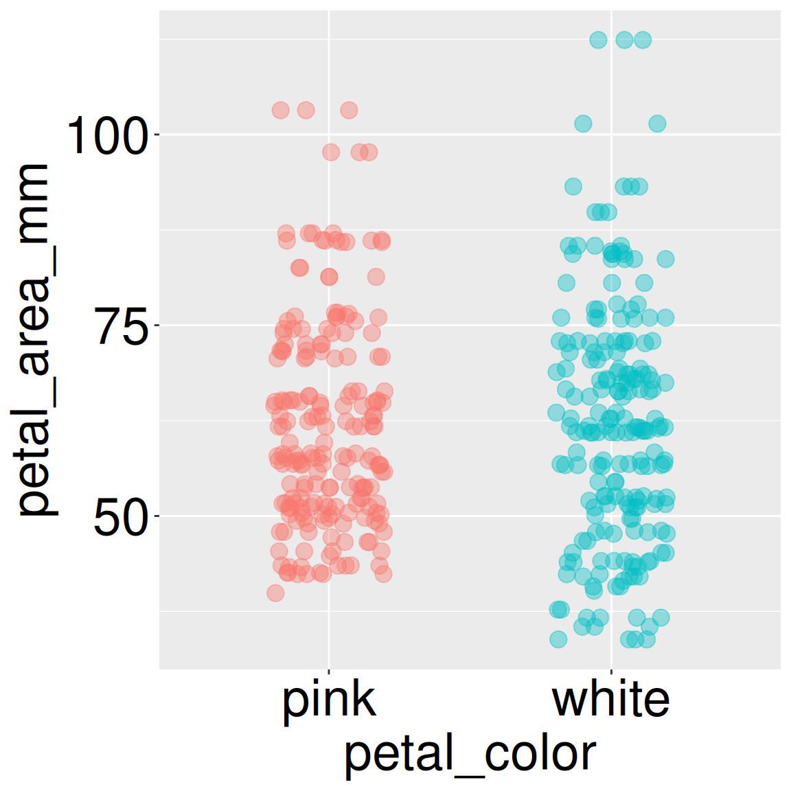
Figure 1: To make sure we have data in regions of parameter space for which we claim an interaction, we make sure our data reasonably covers most combinations of values of explanatory variables.
The one new consideration is that we should be sure that the model actually has the data it needs to solidly infer interactions. So check to see that there is enough data across all combinations of explanatory variables. Figure 1 shows that pink- and white-petaled RILs span roughly similar values of petal area. So this is ok. We’d be more worried if e.g., all very large petals were white.
While this assumption is somewhat distinct from the assumption of no strong multicollinearity, we can see from Figure 1 that the data are not strongly multicollinear.
ASSUMPTION: Data collected without bias. We still believe that data are collected without bias.
ASSUMPTION: Data are independent. We still know data are not fully independent, we have multiple observations per RIL but do not model that. This is not the end of the world and is a great place to start. However, a more proper analysis would include RIL as a “random effect”. I hope to introduce those ideas in the coming chapters. For now we will note this deviation from assumptions and move on.
Assumptions about the shape of the residuals:
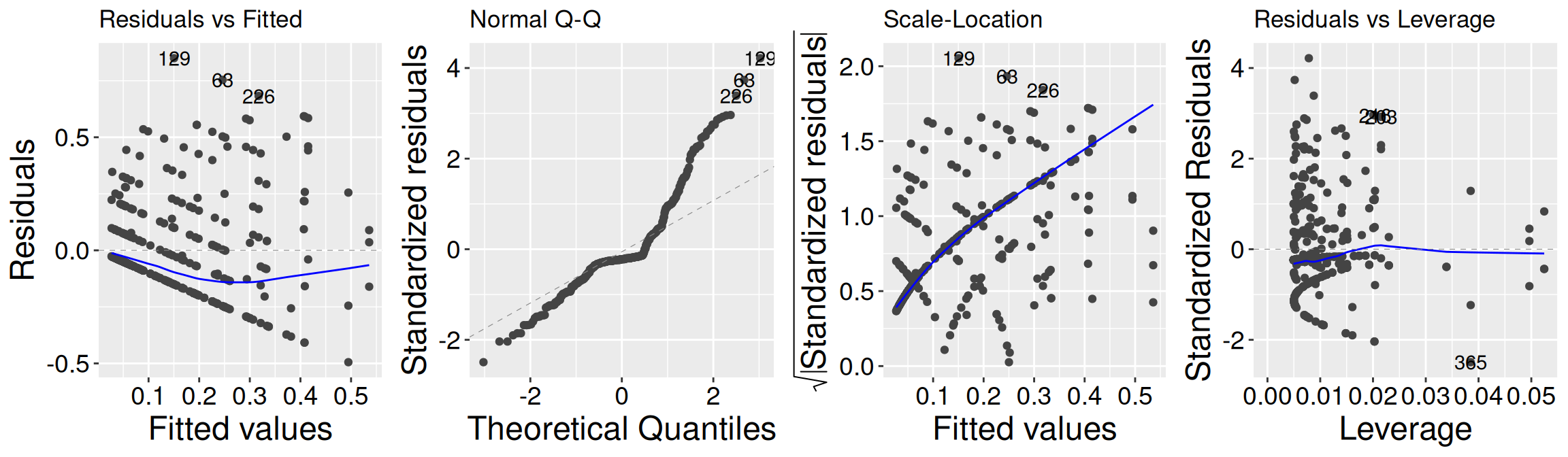
As with all linear models, interaction models make standard assumptions about the structure / shape of residuals. These assumptions relate to how appropriately we are modeling the data, and are best evaluated by visually inspecting diagnostic plots like those in Figure 2.
ASSUMPTION: Normally distributed residuals. The QQ plot (second panel in Figure 2) shows a real deviation from the reference line. This violates assumptions of normality. But, to me, this violation is not super worrying as the sample size is large, and linear models are robust to violations of the normality assumption.
ASSUMPTION: Homoscedasticity. The data also violate the assumption of homoscedasticity. The scale-location plot (third panel in Figure 2) shows this as a positive slope.
ASSUMPTION: Linearity. The residuals-versus-fitted plot in the first panel of Figure 2 shows a slight curved pattern rather than residuals scattered randomly around zero. This suggests that the model may not fully capture the shape of the relationship between the explanatory variables and the response. This all suggests a better model would help, but this isn’t terrible. Because these are bounded proportion data, a model designed for proportions (e.g. logistic regression) or underlying seed counts would be better.
But remember the perfect is the enemy of the good. So for now we move on with caveats. From my experience addressing these deviations from the assumptions improves the model and the specificity of our results. It rarely upends our entire story.
library(ggfortify)autoplot(model, nrow=1)
Figure 2: Diagnostic plots for a linear model of proportion of hybrid seeds as a function of petal area, petal color, and their interaction.
What’s next?
Because interpreting “significance” and the coefficients from an interaction model can be nuanced, we will consider how to responsibly present these results in the next subsection on effect size and uncertainty.