18. Regression

Motivating scenario: You want to know the extent to which a numeric explanatory variable helps predict variation in a numeric response variable. Linear regression lets us model this relationship, estimate its uncertainty, and test the null hypothesis that there is no linear relationship between the variables (i.e. the slope is zero).

Learning goals: By the end of this chapter you should be able to:

Explain the difference between a correlation and a regression slope.
Explain how linear regression models the conditional mean of a response variable as a function of an explanatory variable.
Fit and interpret a simple linear regression.
Use a regression model to predict the value of a continuous response variable from a continuous explanatory variable, and calculate residuals.
Partition variation in a linear regression using sums of squares, and use this to: calculate the F statistic, and test the null hypothesis that the slope is zero.
Use t tests and confidence intervals to estimate uncertainty in the slope and test the null hypothesis that the slope is zero.
Fit, summarize, and interpret linear regression models in R.
Recognize the assumptions, limitations, and common pitfalls of linear regression.

Loading and formatting data

ril_link <- "https://raw.githubusercontent.com/ybrandvain/datasets/refs/heads/master/clarkia_rils.csv"

gc_rils <- readr::read_csv(ril_link) |>
  dplyr::mutate(visited = mean_visits > 0) |>
  filter(location == "GC", !is.na(prop_hybrid), ! is.na(petal_area_mm))|>
  dplyr::select(ril, location, prop_hybrid, petal_area_mm)|>
  mutate(petal_area_quartile = cut( petal_area_mm,
                                    breaks = quantile(petal_area_mm, probs = seq(0, 1, 0.25), na.rm = TRUE),
                                    include.lowest = TRUE))

As biologists, we are often interested in whether one measurement can help predict another. Do plants with larger flowers receive more pollinator visits? Do larger animals produce more offspring? Does temperature predict growth rate? In these cases, we aren’t comparing groups, but rather we ask how variation in an explanatory numeric variable is associated with variation in the response. Lucky for us, the linear model framework can naturally accommodate such cases. In this section, we will investigate how well petal area predicts the proportion of hybrid seeds on parviflora RILs planted at the GC field site.

Why not an ANOVA?

A jittered plot showing proportion hybrid seeds for Clarkia parviflora RILs grouped into four petal-area quartiles. The x-axis shows quartiles Q1 through Q4, and the y-axis shows proportion hybrid seeds from 0 to 1. Most observations in every quartile are near zero, but each quartile also includes some higher values. Red points and vertical error bars show the mean and 95% confidence interval for each quartile, with a dashed line connecting the group means. The group means generally increase from Q1 to Q4, but the binned view is coarse and variable. 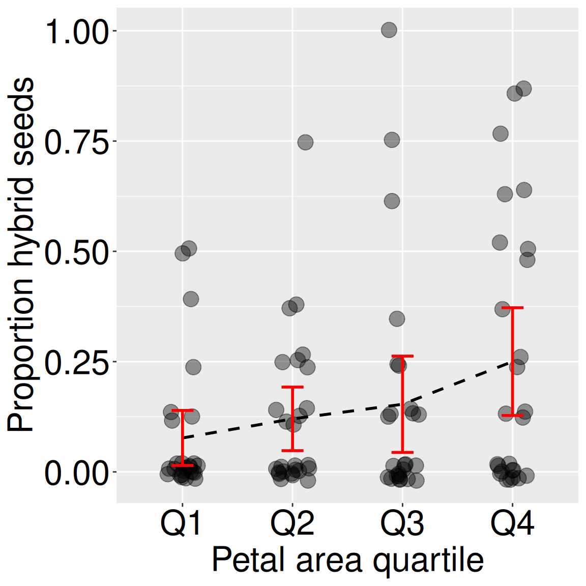— Figure 1: Proportion hybrid seed of parviflora RILs planted at the GC field site as a function of petal area quartile. The quartiles are: Q1: 33.8 – 51.6, Q2: 51.6 – 61.6, Q3: 61.6 – 72.1, Q4: 72.1 – 103.

Of course, we could address this question in a classic ANOVA framework, by binning the x variable into categories. Figure 1 displays this approach: We first bin petal area into quartiles, and then conduct an ANOVA to test the null hypothesis that the proportion of hybrid seeds does not differ as a function of petal area.

This procedure uses three degrees of freedom (one for each model estimate aside from the intercept – Table 1), and does not allow us to reject the null hypothesis (\(p > 0.05\), Table 2). While a fine start, these results are partly a consequence of this modeling decision, not just the underlying relationship in the data.

It makes the same prediction for each observation in a given category, regardless of their precise petal area. These imprecise predictions are both less informative and generate more residual variation than a model that treats x as a true numeric variable.

Table 1) Model coefficients for categorical model.
	coef.qual_model.
(Intercept)	0.077
petal_area:Q2	0.043
petal_area:Q3	0.076
petal_area:Q4	0.173

It spreads the model variation across three degrees of freedom, thereby reducing our power to reject the null hypothesis.

qual_model <- lm(prop_hybrid ~ petal_area_quartile, data = gc_rils)
coef(qual_model)
anova(qual_model)

Table 2) Anova table for categorical model.
	Df	Sum Sq	Mean Sq	F value	Pr(>F)
petal_area_quartile	3	0.422	0.141	2.6	0.056
Residuals	99	5.358	0.054	NA	NA

The answer: A linear regression!

A scatterplot showing proportion hybrid seeds as a function of petal area in square millimeters for Clarkia parviflora RILs at the GC field site. The x-axis shows petal area, ranging roughly from 35 to 105 mm², and the y-axis shows proportion hybrid seeds from 0 to 1. Many observations have hybrid seed proportions near zero, especially at smaller and intermediate petal areas, but higher hybridization values occur more often at larger petal areas. A fitted linear regression line slopes upward, with a gray confidence band that widens toward the edges, indicating a positive association between petal area and proportion hybrid seeds. 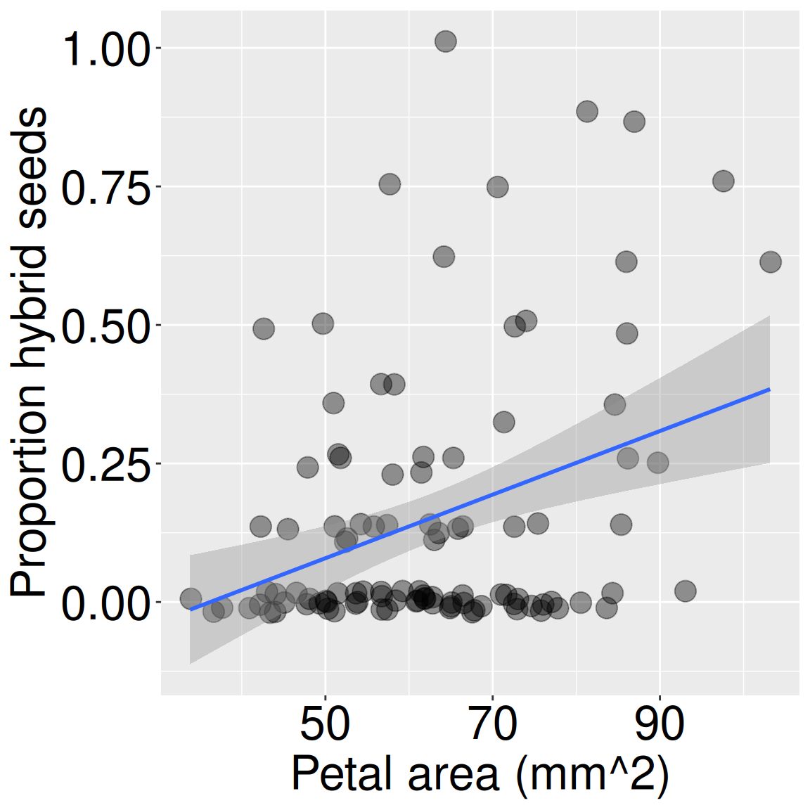— Figure 2: Proportion hybrid seed of parviflora RILs planted at the GC field site by the petal area.

Table 3) Model coefficients for linear regression.
	coef.linear_model.
(Intercept)	-0.20783
petal_area_mm	0.00574

A linear regression circumvents these issues by directly modeling the response variable as a function of the numeric explanatory variable (Figure 2). Thus, each observation gets its own prediction, and the petal-area term uses only one degree of freedom: the slope (Table 3). As a result, we have both a slightly greater model sum of squares than the categorical case, and a much larger model mean square, so we now strongly reject the null hypothesis (Table 4)!

linear_model <- lm(prop_hybrid ~ petal_area_mm, data = gc_rils)
coef(linear_model)
anova(linear_model)

Table 4) Anova table for linear regression.
	Df	Sum Sq	Mean Sq	F value	Pr(>F)
petal_area_mm	1	0.6870	0.6870	13.6224	0.0004
Residuals	101	5.0936	0.0504	NA	NA

What’s Ahead

In this chapter we will consider linear regression

What’s ahead

In this chapter, we will consider linear regression. A linear regression is model for describing how the expected value of a numeric response variable changes with a numeric explanatory variable.

We begin by reviewing three related summaries of association between two numeric variables: covariance, correlation, and slope.
Next, we treat linear regression as a linear model. Just like the models with categorical an explanatory variable and a numeric response, a regression model generates predicted values and residuals. The difference is that regression uses a numeric explanatory variable directly, rather than first sorting observations into groups. We will see how the intercept and slope define the regression line, how to use this line to make predictions, and how to calculate residuals.
Before we get too excited about our model, we will pause to consider assumptions of linear regression. We will also discuss what to do when these assumptions are imperfect, because real biological data rarely behave perfectly.
We then learn to quantify uncertainty in our regression coefficients.
Next, we will learn to test the null hypothesis that the slope equals zero. We will do this in three related ways: with a t-test for the slope, with an ANOVA/F-test based on model and error variation, and with a permutation test that builds a null distribution by shuffling the data.
After that, we will step back and consider caveats in making predictions from linear models. We will see that predictions from linear regression are only trustworthy when they stay close to the range and context of the data used to fit the model.
Finally, we will end with a practical workflow regression in R.

This chapter lays the foundation for the more complex linear models in the remainder of this section.